fox-8/geovista

Cartographic rendering and mesh analytics powered by PyVista

Cartographic rendering and mesh analytics powered by PyVista

⚙️ CI
📈 Health
✨ Meta
📦 Package
🧰 Repo
🛡️ Status

Philisophy

The goal of GeoVista is simple; to complement PyVista with a convenient cartographic capability.

In this regard, from a design perspective we aim to keep GeoVista as pure to PyVista as possible i.e., minimise specialisation as far as practically possible in order to maximise native compatibility within the PyVista and VTK ecosystems.

We intend GeoVista to be a cartographic gateway into the powerful world of PyVista, and all that it offers.

GeoVista is intentionally agnostic to packages such as geopandas, iris, xarray et al, which specialise in preparing your spatial data for visualisation. Rather, we delegate that responsibility and choice of tool to you the user, as we want GeoVista to remain as flexible and open-ended as possible to the entire Scientific Python community.

Simply put, "GeoVista is to PyVista", as "Cartopy is to Matplotlib". Well, that's the aspiration.

Installation

GeoVista is available on both conda-forge and PyPI.

We recommend using conda to install GeoVista 👍

Conda

GeoVista is available on conda-forge, and can be easily installed with conda:

conda install -c conda-forge geovista

or alternatively with mamba:

mamba install -c conda-forge geovista

For more information see our conda-forge feedstock.

Pip

GeoVista is available on PyPI:

pip install geovista[cmap]

Developer

If you simply can't wait for the next release to play with the latest hot features, then you can easily install the main development branch from GitHub:

pip install git+https://github.com/bjlittle/geovista@main

Alternatively, to configure a full developer environment, first clone the GeoVista GitHub repository:

git clone [email protected]:bjlittle/geovista.git

Change to the root directory:

cd geovista

Create the geovista-dev conda development environment for your preferred platform (linux, osx or win) and Python version e.g.,

conda create -n geovista-dev --file requirements/locks/py311-lock-linux-64.txt

Note that, the requirements/locks directory contains fully resolved conda package environments, which are automatically updated on a weekly basis. Alternatively, to get the latest package dependencies, simply:

conda env create --file requirements/geovista.yml

Now activate the environment and install the main development branch of GeoVista:

conda activate geovista-dev
pip install --no-deps --editable .

Finally, you're good to roll 🥳

And for extra credit, install our developer pre-commit git-hooks:

pre-commit install

Quick Start

GeoVista comes with various pre-canned resources to help get you started on your visualisation journey.

Resources

GeoVista makes use of various resources, such as rasters, VTK meshes, Natural Earth features, and sample model data.

If you want to download and cache all registered GeoVista resources to make them available offline, simply:

geovista download --all

Alternatively, just leave GeoVista to download resources on-the-fly, as and when she needs them.

To view the list of registered resources, simply:

geovista download --list

Want to know more?

geovista download --help

Plotting Examples

Let's explore a sample of various oceanographic and atmospheric model data using GeoVista.

WAVEWATCH III

First, let's render a WAVEWATCH III (WW3) unstructured triangular mesh, with 10m Natural Earth coastlines and a 1:50m Natural Earth Cross-Blended Hypsometric Tints base layer.

🗒

import geovista as gv
from geovista.pantry import ww3_global_tri
import geovista.theme

# Load the sample data.
sample = ww3_global_tri()

# Create the mesh from the sample data.
mesh = gv.Transform.from_unstructured(
    sample.lons, sample.lats, connectivity=sample.connectivity, data=sample.data
)

# Plot the mesh.
plotter = gv.GeoPlotter()
sargs = dict(title=f"{sample.name} / {sample.units}")
plotter.add_mesh(
    mesh, show_edges=True, scalar_bar_args=sargs
)
plotter.add_base_layer(texture=gv.natural_earth_hypsometric())
plotter.add_coastlines(resolution="10m")
plotter.view_xy(negative=True)
plotter.add_axes()
plotter.show()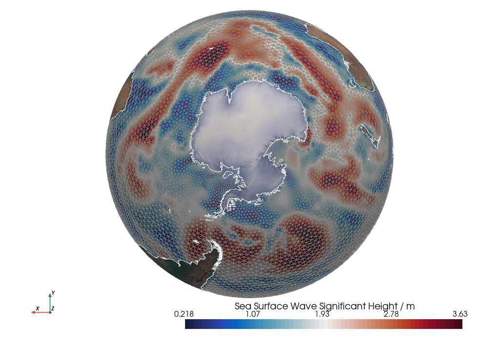

Finite Volume Community Ocean Model

Now, let's visualise the bathymetry of the Plymouth Sound and Tamar River from an FVCOM unstructured mesh, as kindly provided by the Plymouth Marine Laboratory.

🗒

import geovista as gv
from geovista.pantry import fvcom_tamar
import geovista.theme

# Load the sample data.
sample = fvcom_tamar()

# Create the mesh from the sample data.
mesh = gv.Transform.from_unstructured(
    sample.lons,
    sample.lats,
    connectivity=sample.connectivity,
    data=sample.face,
    name="face",
    clean=False,
)

# Warp the mesh nodes by the bathymetry.
mesh.point_data["node"] = sample.node
mesh.compute_normals(cell_normals=False, point_normals=True, inplace=True)
mesh.warp_by_scalar(scalars="node", inplace=True, factor=2e-5)

# Plot the mesh.
plotter = gv.GeoPlotter()
sargs = dict(title=f"{sample.name} / {sample.units}")
plotter.add_mesh(mesh, scalar_bar_args=sargs)
plotter.add_axes()
plotter.show()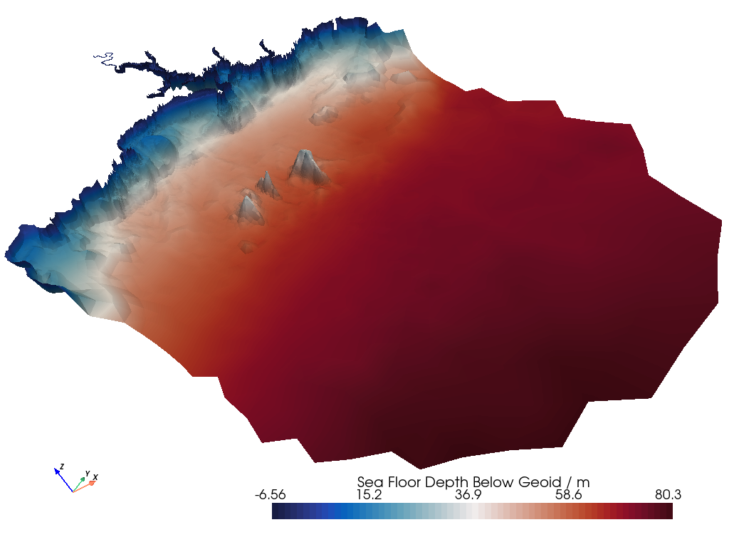

CF UGRID

Local Area Model

Initial projection support is available within GeoVista for Cylindrical and Pseudo-Cylindrical projections. As GeoVista matures and stabilises, we'll aim to complement this capability with other classes of projections, such as Azimuthal and Conic.

In the meantime, let's showcase our basic projection support with some high-resolution unstructured Local Area Model (LAM) data reprojected to Mollweide using a PROJ string, with a 1:50m Natural Earth Cross-Blended Hypsometric Tints base layer.

🗒

import geovista as gv
from geovista.pantry import lam_pacific
import geovista.theme

# Load the sample data.
sample = lam_pacific()

# Create the mesh from the sample data.
mesh = gv.Transform.from_unstructured(
    sample.lons,
    sample.lats,
    connectivity=sample.connectivity,
    data=sample.data,
)

# Plot the mesh on a mollweide projection using a Proj string.
plotter = gv.GeoPlotter(crs="+proj=moll")
sargs = dict(title=f"{sample.name} / {sample.units}")
plotter.add_mesh(mesh, scalar_bar_args=sargs)
plotter.add_base_layer(texture=gv.natural_earth_hypsometric())
plotter.add_axes()
plotter.view_xy()
plotter.show()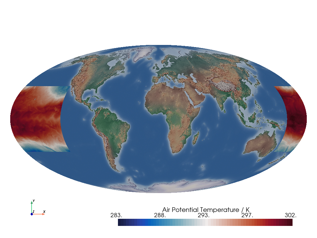

Using the same unstructured LAM data, reproject to Equidistant Cylindrical but this time using a Cartopy Plate Carrée CRS, also with a 1:50m Natural Earth Cross-Blended Hypsometric Tints base layer.

🗒

import cartopy.crs as ccrs

import geovista as gv
from geovista.pantry import lam_pacific
import geovista.theme

# Load the sample data.
sample = lam_pacific()

# Create the mesh from the sample data.
mesh = gv.Transform.from_unstructured(
    sample.lons,
    sample.lats,
    connectivity=sample.connectivity,
    data=sample.data,
)

# Plot the mesh on a Plate Carrée projection using a cartopy CRS.
plotter = gv.GeoPlotter(crs=ccrs.PlateCarree(central_longitude=180))
sargs = dict(title=f"{sample.name} / {sample.units}")
plotter.add_mesh(mesh, scalar_bar_args=sargs)
plotter.add_base_layer(texture=gv.natural_earth_hypsometric())
plotter.add_axes()
plotter.view_xy()
plotter.show()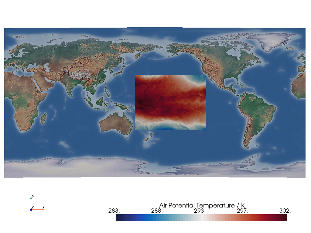

LFRic Cube-Sphere

Now render a Met Office LFRic C48 cube-sphere unstructured mesh of Sea Surface Temperature data on a Robinson projection using an ESRI SRID.

🗒

import geovista as gv
from geovista.pantry import lfric_sst
import geovista.theme

# Load the sample data.
sample = lfric_sst()

# Create the mesh from the sample data.
mesh = gv.Transform.from_unstructured(
    sample.lons,
    sample.lats,
    connectivity=sample.connectivity,
    data=sample.data,
)

# Plot the mesh on a Robinson projection using an ESRI spatial reference identifier.
plotter = gv.GeoPlotter(crs="ESRI:54030")
sargs = dict(title=f"{sample.name} / {sample.units}")
plotter.add_mesh(mesh, cmap="thermal", show_edges=True, scalar_bar_args=sargs)
plotter.view_xy()
plotter.add_axes()
plotter.show()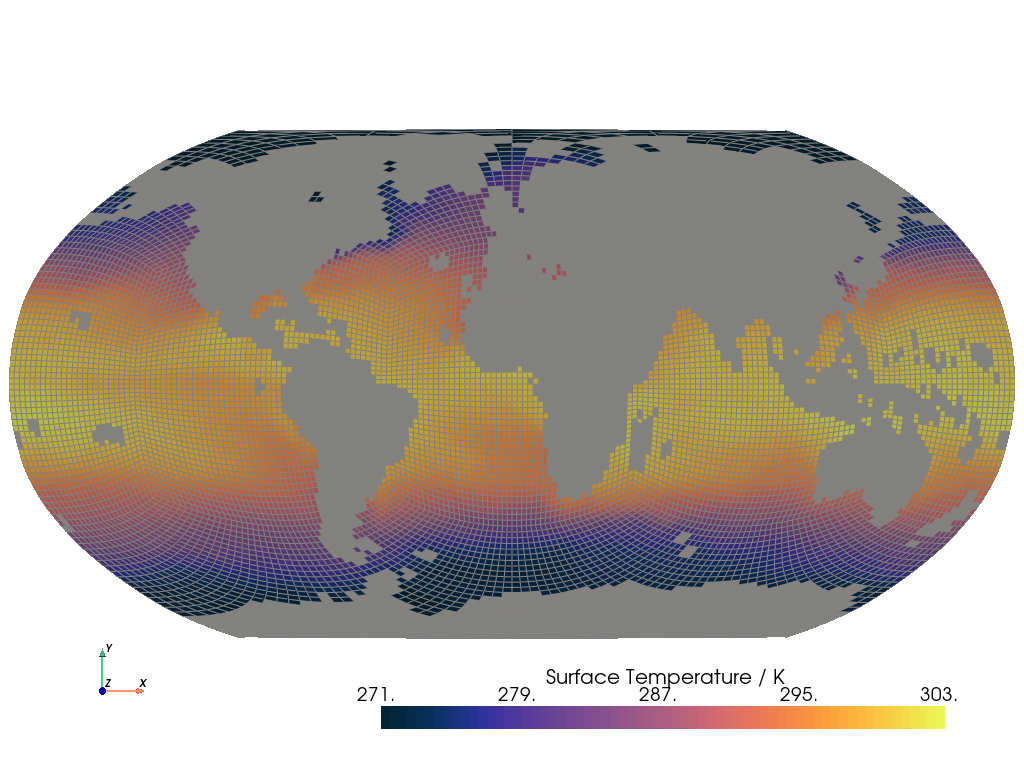

UM ORCA2

So far we've demonstrated GeoVista's ability to cope with unstructured data. Now let's plot a curvilinear mesh using Met Office Unified Model (UM) ORCA2 Sea Water Potential Temperature data, with 10m Natural Earth coastlines and a 1:50m Natural Earth I base layer.

🗒

import geovista as gv
from geovista.pantry import um_orca2
import geovista.theme

# Load sample data.
sample = um_orca2()

# Create the mesh from the sample data.
mesh = gv.Transform.from_2d(sample.lons, sample.lats, data=sample.data)

# Remove cells from the mesh with NaN values.
mesh = mesh.threshold()

# Plot the mesh.
plotter = gv.GeoPlotter()
sargs = dict(title=f"{sample.name} / {sample.units}")
plotter.add_mesh(
    mesh, show_edges=True, scalar_bar_args=sargs
)
plotter.add_base_layer(texture=gv.natural_earth_1())
plotter.add_coastlines(resolution="10m")
plotter.view_xy()
plotter.add_axes()
plotter.show()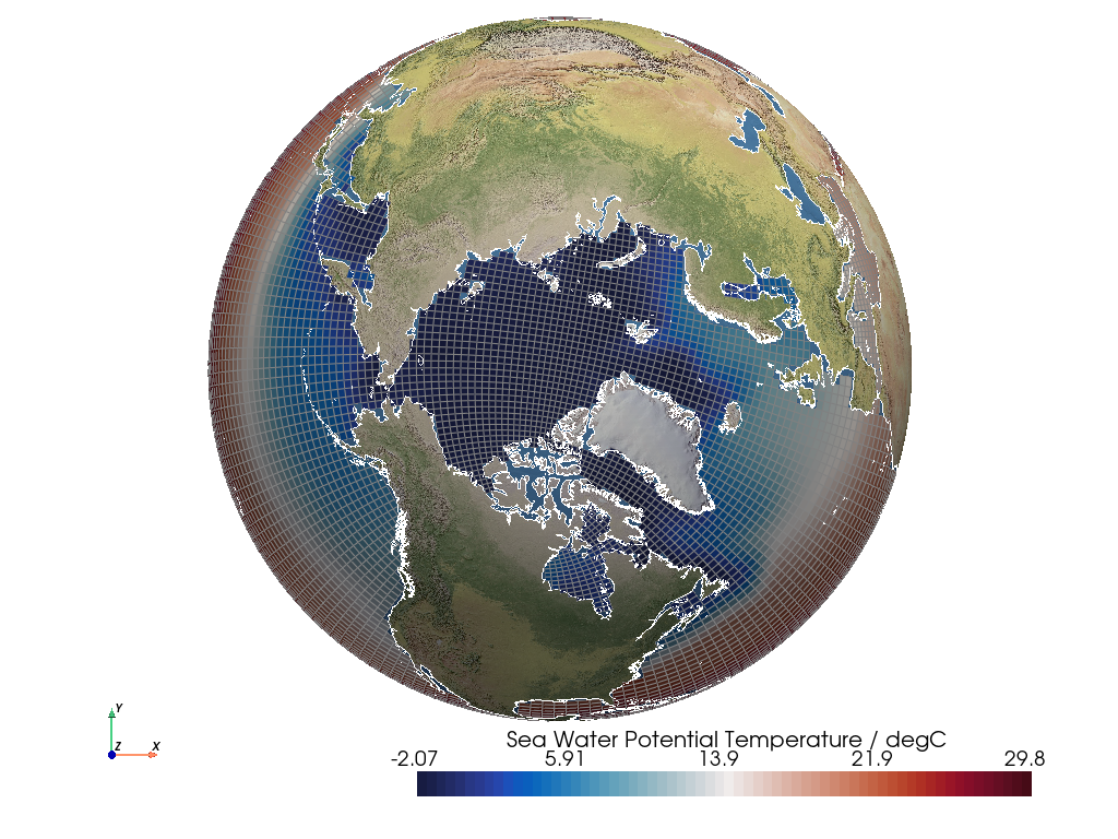

OISST AVHRR

Finally, let's render a NOAA/NCEI Optimum Interpolation SST (OISST) Advanced Very High Resolution Radiometer (AVHRR) rectilinear mesh, with 10m Natural Earth coastlines and a NASA Blue Marble base layer.

🗒

import geovista as gv
from geovista.pantry import oisst_avhrr_sst
import geovista.theme

# Load sample data.
sample = oisst_avhrr_sst()

# Create the mesh from the sample data.
mesh = gv.Transform.from_1d(sample.lons, sample.lats, data=sample.data)

# Remove cells from the mesh with NaN values.
mesh = mesh.threshold()

# Plot the mesh.
plotter = gv.GeoPlotter()
sargs = dict(title=f"{sample.name} / {sample.units}")
plotter.add_mesh(mesh, scalar_bar_args=sargs)
plotter.add_base_layer(texture=gv.blue_marble())
plotter.add_coastlines()
plotter.view_xz()
plotter.add_axes()
plotter.show()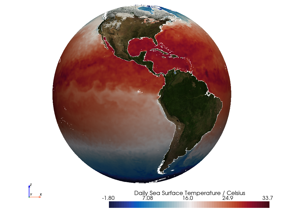

Further Examples

"Please, sir, I want some more", Charles Dickens, Oliver Twist, 1838.

Certainly, our pleasure! From the command line, simply:

geovista examples --run all --verbose

Want to know more?

geovista examples --help

Further Reading

Whilst you're here, why not hop on over to the pyvista-xarray project and check it out!

It's aiming to provide xarray DataArray accessors for PyVista to visualize datasets in 3D for the xarray community, and will be building on top of GeoVista 🎉

License

GeoVista is distributed under the terms of the BSD-3-Clause license.

#ShowYourStripes

Graphics and Lead Scientist: Ed Hawkins, National Centre for Atmospheric Science, University of Reading.

Data: Berkeley Earth, NOAA, UK Met Office, MeteoSwiss, DWD, SMHI, UoR, Meteo France & ZAMG.

#ShowYourStripes is distributed under a Creative Commons Attribution 4.0 International License