anguoyang/phy-net

compressing physics with neural networks

Phy-Net

Introduction

This repository is a look at compressing Lattice Boltzmann physics simulations onto neural networks. This approach relies on learning a compressed representation of simulation while learning the dynamics on this compressed form. This allows us to simulate large systems with low memory and computation. Here is a rough draft of the paper.

Related Work

Similar works can be found in "Accelerating Eulerian Fluid Simulation With Convolutional Networks" and "Convolutional Neural Networks for steady Flow Approximation".

Network Details

The network learns a encoding, compression, and decoding piece. The encoding piece learns to compress the state of the physics simulation. The compression piece learns the dynamics of the simulation on this compressed piece. The decoding piece learns to decode the compressed representation. The network is kept all convolutional allowing it to be trained and evaluated on any size simulation. This means that once the model is trained on a small simulation (say 256 by 256 grid) it can then attempt to simulate the dynamics of a larger simulation (say 1024 by 1024 grid). We show that the model can still produce accurate results even with larger simulations then seen during training.

Lattice Boltzmann Fluid Flow

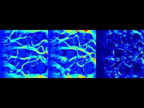
Using the Mechsys library we generated 2D and 3D fluid simulations to train our model. For the 2D case we simulate a variety of random objects interacting with a steady flow and periodic boundary conditions. The simulation is a 256 by 256 grid. Using the trained model we evaluate on grid size 256 by 256, 512 by 512, and 1024 by 1024. Here are examples of generated simulations (network design is being iterated on).

We can look at various properties of the true versus generated simulations such as mean squared error, divergence of the velocity vector field, drag, and flux. Averaging over several test simulations we see the that the generated simulation produces realistic values. The following graphs show this for 256, 512, and 1024 sized simulations.

We notice that the model produces lower then expected y flux for both the 512 and 1024 simulations. This is understandable because the larger simulations tend to have higher y flows then smaller simulations due to the distribution of objects being more clumped. It appears that this effect can be mitigated by changing the object density and distribution (under investigation).

A few more snap shots of simulations

Now we can apply it to other datasets. Check this out!

Here are some 3D simulations

Here are the plots for the 3D simulations. There may be a bug in how the drag is calculated right now.

Lattice Boltzmann Electromagnetic Waves

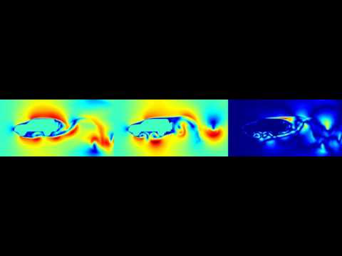
Well the Lattice Boltzmann method is actually a general partial differential equation solver (of a particular form) so why stop at fluid flow! Here are some fun electromagnetic simulations that the model learns! These simulations are of a wave hitting randomly placed objects with different dielectric constants. You can see fun effects such as reflection and refraction when the wave interacts with the surface.

Here are the plots for EM simulations

How to run

Running the 2d simulations requires around 100 Gb of hard drive memory, a good gpu (currently using GTX 1080s), and 1 and a half days.

Generating Data

The test and train sets are generated using the Mechsys library. Follow the installation guild found here. Once the directory is unpacked run ccmake . followed by c. Then scroll to the flag that says A_USE_OCL and hit enter to raise the flag. Press c again to configure followed by g to generate (I found ccmake to be confusing at first). Quit the prompt and run make. Now copy the contents of Phy-Net/systems/mechsys_fluid_flow to the directory mechsys/tflbm. Now enter mechsys/tflbm and run make followed by

./generate_data.

This will generate the required train and test set for the 2D simulations and save them to /data/ (this can be changed in the run_bunch_2d script. 3D simulation is commented out for now. Generating the 2D simulation data will require about 12 hours.

Train Model

To train the model enter the Phy-Net/train directory and run

python compress_train.py

This will first generate tfrecords for the generated training data and then begin training. Multi GPU training is supported with the flag --nr_gpu=n for n gpus. The important flags for training and model configurations are

• --nr_residual=2 Number of residual blocks in each downsample chunk of the encoder and decoder
• --nr_downsamples=4 Number of downsamples in the encoder and decoder
• --filter_size=8 Number of filters for the first encoder layer. The filters double after each downsample.
• --nr_residual_compression=3 Number of residual blocks in compression peice.
• --filter_size_compression=64 filter size of residual blocks in compression peice.
• --unroll_length=5 Number of steps in the future the network is unrolled.

All flags and their uses can be found in Phy-Net/model/ring_net.py.

Test Model

There are 4 different tests that can be run.

• run_2d_error_script Generates the error plots seen above
• run_2d_image_script Generates the images seen above
• run_2d_video_script Generates the videos seen above
• runtime_script Generates benchmarks for run times

TODO

• Stream line data generation process

Simplifing the data generation process with a script would be nice. It seems reasonable that there could be a script that downloads and compiles mechsys as well as moves the necessary files around.

• Train model effectively on 3D simulations

The 3D simulations are not training effectively yet. The attempts made so far are,

1. Reducing Reynolds number. The Reynolds number appeared to be to high making the simulations extremely chaotic and thus hard to learn. Lowering it seems to have helped convergence and accuracy.
2. Made all objects spheres of the same size. Not sure how much of an effect this has had. Once the network trains on these simulations effectively we will try more diverse datasets.
3. larger network with filter size 64 and compression filter size 256. Seems to slow down training and cause over fitting.

• Test extracting state

A key peice of this work is the ability to extract out only a desired part of the compressed state to make measurements on. This is required because extracting the full state requires just as much memory as simulating and thus makes the compression aspect of this method useless. You should be able to extract small chunch of the full simulation from the compressed state.

Still flushing out list

Conclusion

This project is under active development.