antouank/d3-shape

Graphical primitives for visualization, such as lines and areas.

d3-shape

Visualizations typically consist of discrete graphical marks, such as symbols, arcs, lines and areas. While the rectangles of a bar chart may be easy enough to generate directly using SVG or Canvas, other shapes are complex, such as rounded annular sectors and centripetal Catmull–Rom splines. This module provides a variety of shape generators for your convenience.

As with other aspects of D3, these shapes are driven by data: each shape generator exposes accessors that control how the input data are mapped to a visual representation. For example, you might define a line generator for a time series by linearly scaling the date and value fields of your data to fit the chart:

var l = line()
    .x(function(d) { return x(d.date); })
    .y(function(d) { return y(d.value); })
    .curve(shape.catmullRom);

The line generator can then be used to set the d attribute of an SVG path element:

path.datum(data).attr("d", l);

Or you can use it to render to a Canvas 2D context:

l.context(context)(data);

Installing

If you use NPM, npm install d3-shape. Otherwise, download the latest release.

API Reference

Arcs

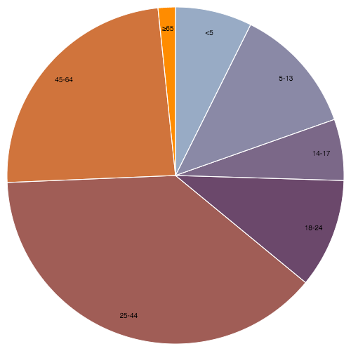
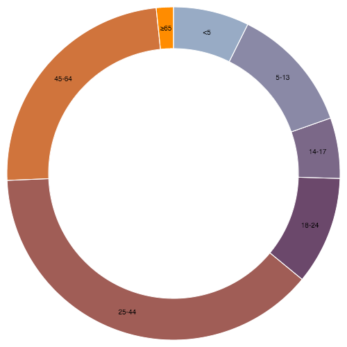
The arc generator produces a circular or annular sector, as in a pie or donut chart. If the difference between the start and end angles (the angular span) is greater than τ, the arc generator will produce a complete circle or annulus. If it is less than τ, arcs may have rounded corners and angular padding. Arcs are always centered at ⟨0,0⟩; use a transform (see: SVG, Canvas) to move the arc to a different position.

See also the pie generator, which computes the necessary angles to represent an array of data as a pie or donut chart; these angles can then be passed to an arc generator.

# arc()

Constructs a new arc generator with the default settings.

# arc(arguments…)

Generates an arc for the given arguments. The arguments are arbitrary; they are simply propagated to the arc generator’s accessor functions along with the this object. For example, with the default settings, an object with radii and angles is expected:

var a = arc();

a({
  innerRadius: 0,
  outerRadius: 100,
  startAngle: 0,
  endAngle: Math.PI / 2
}); // "M0,-100A100,100,0,0,1,100,0L0,0Z"

If the radii and angles are instead defined as constants, you can generate an arc without any arguments:

var a = arc()
    .innerRadius(0)
    .outerRadius(100)
    .startAngle(0)
    .endAngle(Math.PI / 2);

a(); // "M0,-100A100,100,0,0,1,100,0L0,0Z"

If the arc generator has a context, then the arc is rendered to this context as a sequence of path method calls and this function returns void. Otherwise, a path data string is returned.

# arc.centroid(arguments…)

Computes the midpoint [x, y] of the center line of the arc that would be generated by the given arguments. The arguments are arbitrary; they are simply propagated to the arc generator’s accessor functions along with the this object. To be consistent with the generated arc, the accessors must be deterministic, i.e., return the same value given the same arguments. The midpoint is defined as (startAngle + endAngle) / 2 and (innerRadius + outerRadius) / 2. For example:

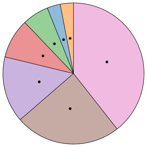
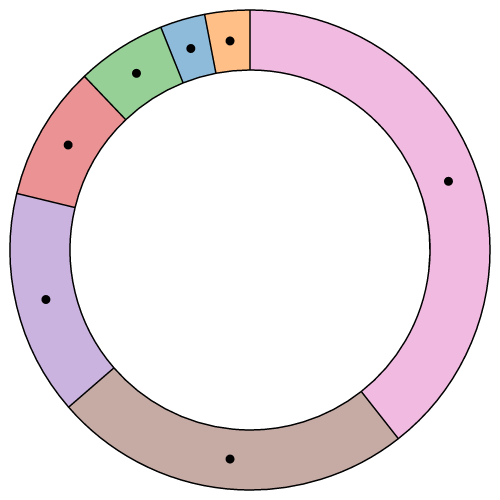
Note that this is not the geometric center of the arc, which may be outside the arc; this method is merely a convenience for positioning labels.

# arc.innerRadius([radius])

If radius is specified, sets the inner radius to the specified function or number and returns this arc generator. If radius is not specified, returns the current inner radius accessor, which defaults to:

function innerRadius(d) {
  return d.innerRadius;
}

Specifying the inner radius as a function is useful for constructing a stacked polar bar chart, often in conjunction with a sqrt scale. More commonly, a constant inner radius is used for a donut or pie chart. If the outer radius is smaller than the inner radius, the inner and outer radii are swapped. A negative value is treated as zero.

# arc.outerRadius([radius])

If radius is specified, sets the outer radius to the specified function or number and returns this arc generator. If radius is not specified, returns the current outer radius accessor, which defaults to:

function outerRadius(d) {
  return d.outerRadius;
}

Specifying the outer radius as a function is useful for constructing a coxcomb or polar bar chart, often in conjunction with a sqrt scale. More commonly, a constant outer radius is used for a pie or donut chart. If the outer radius is smaller than the inner radius, the inner and outer radii are swapped. A negative value is treated as zero.

# arc.cornerRadius([radius])

If radius is specified, sets the corner radius to the specified function or number and returns this arc generator. If radius is not specified, returns the current corner radius accessor, which defaults to:

function cornerRadius() {
  return 0;
}

If the corner radius is greater than zero, the corners of the arc are rounded using circles of the given radius. For a circular sector, the two outer corners are rounded; for an annular sector, all four corners are rounded. The corner circles are shown in this diagram:

The corner radius may not be larger than (outerRadius - innerRadius) / 2. In addition, for arcs whose angular span is less than π, the corner radius may be reduced as two adjacent rounded corners intersect. This is occurs more often with the inner corners. See the arc corners animation for illustration.

# arc.startAngle([angle])

If angle is specified, sets the start angle to the specified function or number and returns this arc generator. If angle is not specified, returns the current start angle accessor, which defaults to:

function startAngle(d) {
  return d.startAngle;
}

The angle is specified in radians, with 0 at -y (12 o’clock) and positive angles proceeding clockwise. If |endAngle - startAngle| ≥ τ, a complete circle or annulus is generated rather than a sector.

# arc.endAngle([angle])

If angle is specified, sets the end angle to the specified function or number and returns this arc generator. If angle is not specified, returns the current end angle accessor, which defaults to:

function endAngle(d) {
  return d.endAngle;
}

The angle is specified in radians, with 0 at -y (12 o’clock) and positive angles proceeding clockwise. If |endAngle - startAngle| ≥ τ, a complete circle or annulus is generated rather than a sector.

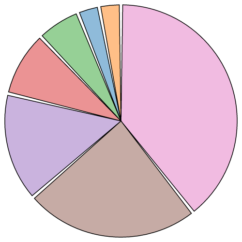
# arc.padAngle([angle])

If angle is specified, sets the pad angle to the specified function or number and returns this arc generator. If angle is not specified, returns the current pad angle accessor, which defaults to:

function padAngle() {
  return d && d.padAngle;
}

The pad angle is converted to a fixed linear distance separating adjacent arcs, defined as padRadius * padAngle. This distance is subtracted equally from the start and end of the arc. If the arc forms a complete circle or annulus, as when |endAngle - startAngle| ≥ τ, the pad angle is ignored.

If the inner radius or angular span is small relative to the pad angle, it may not be possible to maintain parallel edges between adjacent arcs. In this case, the inner edge of the arc may collapse to a point, similar to a circular sector. For this reason, padding is typically only applied to annular sectors (i.e., when innerRadius is positive), as shown in this diagram:

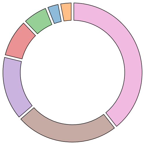
The recommended minimum inner radius when using padding is outerRadius * padAngle / sin(θ), where θ is the angular span of the smallest arc before padding. For example, if the outer radius is 200 pixels and the pad angle is 0.02 radians, a reasonable θ is 0.04 radians, and a reasonable inner radius is 100 pixels. See the arc padding animation for illustration.

Often, the pad angle is not set directly on the arc generator, but is instead computed by the pie generator so as to ensure that the area of padded arcs is proportional to their value; see pie.padAngle. See the pie padding animation for illustration. If you apply a constant pad angle to the arc generator directly, it tends to subtract disproportionately from smaller arcs, introducing distortion.

# arc.padRadius([radius])

If radius is specified, sets the pad radius to the specified function or number and returns this arc generator. If radius is not specified, returns the current pad radius accessor, which defaults to null, indicating that the pad radius should be automatically computed as sqrt(innerRadius * innerRadius + outerRadius * outerRadius). The pad radius determines the fixed linear distance separating adjacent arcs, defined as padRadius * padAngle.

# arc.context([context])

If context is specified, sets the context and returns this arc generator. If context is not specified, returns the current context, which defaults to null. If the context is not null, then the generated arc is rendered to this context as a sequence of path method calls. Otherwise, a path data string representing the generated arc is returned.

Pies

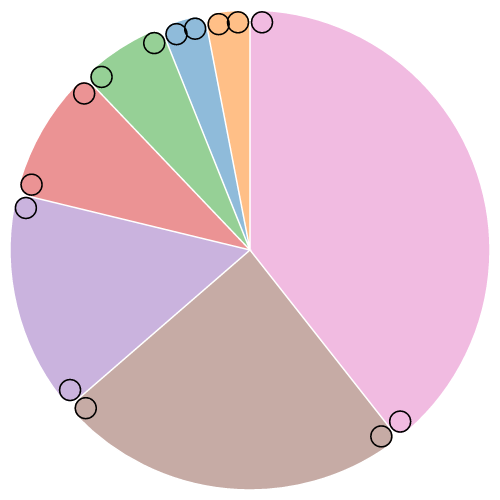
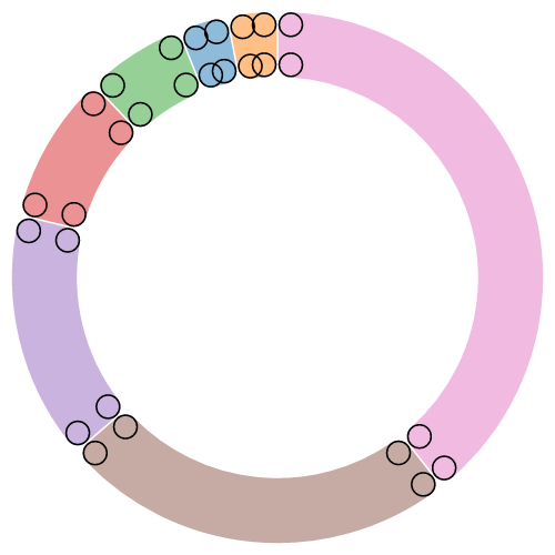
The pie generator does not produce a shape directly, but instead computes the necessary angles to represent a tabular dataset as a pie or donut chart; these angles can then be passed to an arc generator.

# pie()

Constructs a new pie generator with the default settings.

# pie(data[, arguments…])

Generates a pie for the given array of data, returning an array of objects representing each datum’s arc angles. Any additional arguments are arbitrary; they are simply propagated to the pie generator’s accessor functions along with the this object. The length of the returned array is the same as data, and each element i in the returned array corresponds to the element i in the input data. Each object in the returned array has the following properties:

• data - the input datum; the corresponding element in the input data array.
• value - the numeric value of the arc.
• startAngle - the start angle of the arc.
• endAngle - the end angle of the arc.
• padAngle - the pad angle of the arc.

This representation is designed to work with the arc generator’s default startAngle, endAngle and padAngle accessors. The angular units are arbitrary, but if you plan to use the pie generator in conjunction with an arc generator, you should specify angles in radians, with 0 at -y (12 o’clock) and positive angles proceeding clockwise.

Given a small dataset of numbers, here is how to compute the arc angles to render this data as a pie chart:

var data = [1, 1, 2, 3, 5, 8, 13, 21];
var arcs = pie()(data);

The first pair of parens, pie(), constructs a default pie generator. The second, pie()(data), invokes this generator on the dataset, returning an array of objects:

[
  {"data":  1, "value":  1, "startAngle": 6.050474740247008, "endAngle": 6.166830023713296, "padAngle": 0},
  {"data":  1, "value":  1, "startAngle": 6.166830023713296, "endAngle": 6.283185307179584, "padAngle": 0},
  {"data":  2, "value":  2, "startAngle": 5.817764173314431, "endAngle": 6.050474740247008, "padAngle": 0},
  {"data":  3, "value":  3, "startAngle": 5.468698322915565, "endAngle": 5.817764173314431, "padAngle": 0},
  {"data":  5, "value":  5, "startAngle": 4.886921905584122, "endAngle": 5.468698322915565, "padAngle": 0},
  {"data":  8, "value":  8, "startAngle": 3.956079637853813, "endAngle": 4.886921905584122, "padAngle": 0},
  {"data": 13, "value": 13, "startAngle": 2.443460952792061, "endAngle": 3.956079637853813, "padAngle": 0},
  {"data": 21, "value": 21, "startAngle": 0.000000000000000, "endAngle": 2.443460952792061, "padAngle": 0}
]

Note that the returned array is in the same order as the data, even though this pie chart is sorted by descending value, starting with the arc for the last datum (value 21) at 12 o’clock.

# pie.value([value])

If value is specified, sets the value accessor to the specified function or number and returns this pie generator. If value is not specified, returns the current value accessor, which defaults to:

function value(d) {
  return d;
}

When a pie is generated, the value accessor will be invoked for each element in the input data array, being passed the element d, the index i, and the array data as three arguments. The default value accessor assumes that the input data are numbers, or that they are coercible to numbers using valueOf. If your data are not simply numbers, then you should specify an accessor that returns the corresponding numeric value for a given datum. For example:

var data = [
  {"number":  4, "name": Locke},
  {"number":  8, "name": Reyes},
  {"number": 15, "name": Ford},
  {"number": 16, "name": Jarrah},
  {"number": 23, "name": Shephard},
  {"number": 42, "name": Kwon}
];

var arcs = pie()
    .value(function(d) { return d.number; })
    (data);

This is similar to mapping your data to values before invoking the pie generator:

var arcs = pie()(data.map(function(d) { return d.number; }));

The benefit of an accessor is that the input data remains associated with the returned objects, thereby making it easier to access other fields of the data, for example to set the color or to add text labels.

# pie.sort([compare])

If compare is specified, sets the data comparator to the specified function and returns this pie generator. If compare is not specified, returns the current data comparator, which defaults to null. If both the data comparator and the value comparator are null, then arcs are positioned in the original input order. Otherwise, the data is sorted according to the data comparator, and the resulting order is used. Setting the data comparator implicitly sets the value comparator to null.

The compare function takes two arguments a and b, each elements from the input data array. If the arc for a should be before the arc for b, then the comparator must return a number less than zero; if the arc for a should be after the arc for b, then the comparator must return a number greater than zero; returning zero means that the relative order of a and b is unspecified. For example, to sort arcs by their associated name:

pie.sort(function(a, b) { return a.name.localeCompare(b.name); });

Sorting does not affect the order of the generated arc array which is always in the same order as the input data array; it merely affects the computed angles of each arc. The first arc starts at the start angle and the last arc ends at the end angle.

# pie.sortValues([compare])

If compare is specified, sets the value comparator to the specified function and returns this pie generator. If compare is not specified, returns the current value comparator, which defaults to descending value. The default value comparator is implemented as:

function compare(a, b) {
  return b - a;
}

If both the data comparator and the value comparator are null, then arcs are positioned in the original input order. Otherwise, the data is sorted according to the data comparator, and the resulting order is used. Setting the value comparator implicitly sets the data comparator to null.

The value comparator is similar to the data comparator, except the two arguments a and b are values derived from the input data array using the value accessor, not the data elements. If the arc for a should be before the arc for b, then the comparator must return a number less than zero; if the arc for a should be after the arc for b, then the comparator must return a number greater than zero; returning zero means that the relative order of a and b is unspecified. For example, to sort arcs by ascending value:

pie.sortValues(function(a, b) { return a - b; });

Sorting does not affect the order of the generated arc array which is always in the same order as the input data array; it merely affects the computed angles of each arc. The first arc starts at the start angle and the last arc ends at the end angle.

# pie.startAngle([angle])

If angle is specified, sets the overall start angle of the pie to the specified function or number and returns this pie generator. If angle is not specified, returns the current start angle accessor, which defaults to:

function startAngle() {
  return 0;
}

The start angle here means the overall start angle of the pie, i.e., the start angle of the first arc. The start angle accessor is invoked once, being passed the same arguments and this context as the pie generator. The units of angle are arbitrary, but if you plan to use the pie generator in conjunction with an arc generator, you should specify an angle in radians, with 0 at -y (12 o’clock) and positive angles proceeding clockwise.

# pie.endAngle([angle])

If angle is specified, sets the overall end angle of the pie to the specified function or number and returns this pie generator. If angle is not specified, returns the current end angle accessor, which defaults to:

function endAngle() {
  return 2 * Math.PI;
}

The end angle here means the overall end angle of the pie, i.e., the end angle of the last arc. The end angle accessor is invoked once, being passed the same arguments and this context as the pie generator. The units of angle are arbitrary, but if you plan to use the pie generator in conjunction with an arc generator, you should specify an angle in radians, with 0 at -y (12 o’clock) and positive angles proceeding clockwise.

The value of the end angle is constrained to startAngle ± τ, such that |endAngle - startAngle| ≤ τ.

# pie.padAngle([angle])

If angle is specified, sets the pad angle to the specified function or number and returns this pie generator. If angle is not specified, returns the current pad angle accessor, which defaults to:

function padAngle() {
  return 0;
}

The pad angle here means the angular separation between each adjacent arc. The total amount of padding reserved is the specified angle times the number of elements in the input data array, and at most |endAngle - startAngle|; the remaining space is then divided proportionally by value such that the relative area of each arc is preserved. See the pie padding animation for illustration. The pad angle accessor is invoked once, being passed the same arguments and this context as the pie generator. The units of angle are arbitrary, but if you plan to use the pie generator in conjunction with an arc generator, you should specify an angle in radians.

Lines

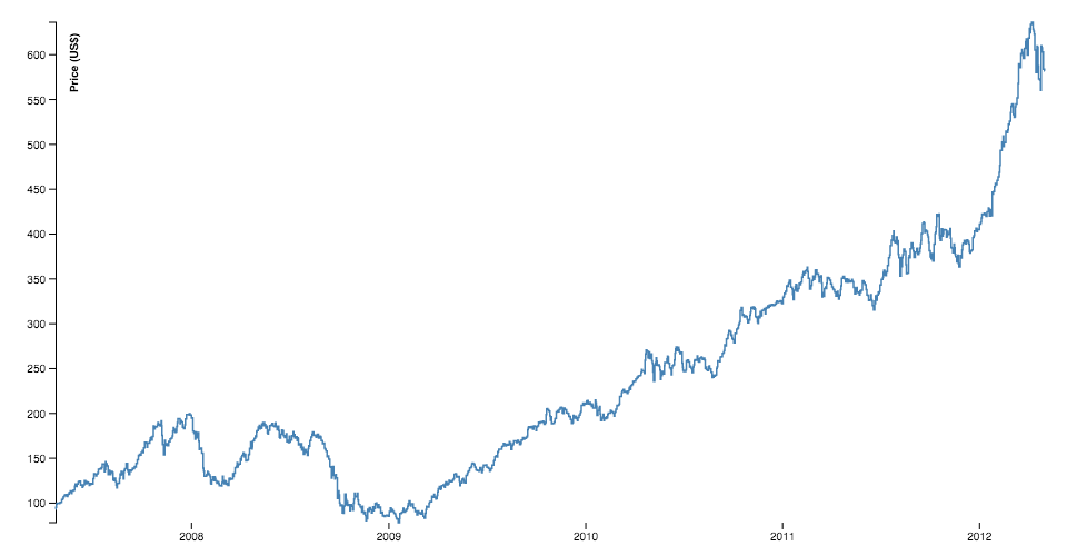
The line generator produces a spline or polyline, as in a line chart. Lines also appear in many other visualization types, such as the links in hierarchical edge bundling.

# line()

Constructs a new line generator with the default settings.

# line(data)

Generates a line for the given array of data. Depending on this line generator’s associated curve, the given input data may need to be sorted by x-value before being passed to the line generator. If the line generator has a context, then the line is rendered to this context as a sequence of path method calls and this function returns void. Otherwise, a path data string is returned.

# line.x([x])

If x is specified, sets the x accessor to the specified function or number and returns this line generator. If x is not specified, returns the current x accessor, which defaults to:

function x(d) {
  return d[0];
}

When a line is generated, the x accessor will be invoked for each defined element in the input data array, being passed the element d, the index i, and the array data as three arguments. The default x accessor assumes that the input data are two-element arrays of numbers. If your data are in a different format, or if you wish to transform the data before rendering, then you should specify a custom accessor. For example, if x is a time scale and y is a linear scale:

var data = [
  {date: new Date(2007, 3, 24), value: 93.24},
  {date: new Date(2007, 3, 25), value: 95.35},
  {date: new Date(2007, 3, 26), value: 98.84},
  {date: new Date(2007, 3, 27), value: 99.92},
  {date: new Date(2007, 3, 30), value: 99.80},
  {date: new Date(2007, 4,  1), value: 99.47},
  …
];

var l = line()
    .x(function(d) { return x(d.date); })
    .y(function(d) { return y(d.value); });

This is similar to mapping your data to values before invoking the line generator:

line()(data.map(function(d) { return [x(d.date), y(d.value)]; }));

The benefit of an accessor is that the input data remains associated with the returned objects, thereby making it easier to access other fields of the data, for example to set the color or to add text labels.

# line.y([y])

If y is specified, sets the y accessor to the specified function or number and returns this line generator. If y is not specified, returns the current y accessor, which defaults to:

function y(d) {
  return d[1];
}

When a line is generated, the y accessor will be invoked for each defined element in the input data array, being passed the element d, the index i, and the array data as three arguments. The default y accessor assumes that the input data are two-element arrays of numbers. See line.x for more information.

# line.defined([defined])

If defined is specified, sets the defined accessor to the specified function or boolean and returns this line generator. If defined is not specified, returns the current defined accessor, which defaults to:

function defined() {
  return true;
}

The default accessor thus assumes that the input data is always defined. When a line is generated, the defined accessor will be invoked for each element in the input data array, being passed the element d, the index i, and the array data as three arguments. If the given element is defined (i.e., if the defined accessor returns a truthy value for this element), the x and y accessors will subsequently be evaluated and the point will be added to the current line segment. Otherwise, the element will be skipped, the current line segment will be ended, and a new line segment will be generated for the next defined point. As a result, the generated line may have several discrete segments. For example:

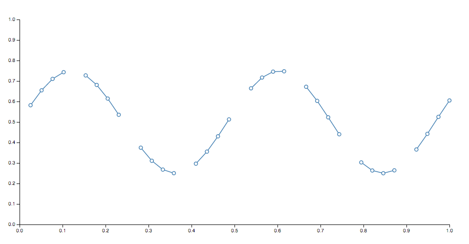
Note that if a line segment consists of only a single point, it may appear invisible unless rendered with rounded or square line caps. In addition, some curves such as cardinalOpen only render a visible segment if it contains multiple points.

# line.curve([curve[, parameters…]])

If curve is specified, sets the curve factory and returns this line generator. Any optional parameters, if specified, will be bound to the specified curve. If curve is not specified, returns the current curve factory, which defaults to linear.

# line.context([context])

If context is specified, sets the context and returns this line generator. If context is not specified, returns the current context, which defaults to null. If the context is not null, then the generated line is rendered to this context as a sequence of path method calls. Otherwise, a path data string representing the generated line is returned.

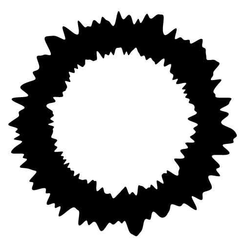
# radialLine()

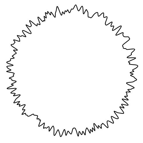
Constructs a new radial line generator with the default settings. A radial line generator is equivalent to the standard Cartesian line generator, except the x and y accessors are replaced with angle and radius accessors. Radial lines are always positioned relative to ⟨0,0⟩; use a transform (see: SVG, Canvas) to change the origin.

# radialLine.angle([angle])

Equivalent to line.x, except the accessor returns the angle in radians, with 0 at -y (12 o’clock).

# radialLine.radius([radius])

Equivalent to line.y, except the accessor returns the radius: the distance from the origin ⟨0,0⟩.

# radialLine.defined([defined])

Equivalent to line.defined.

# radialLine.curve([curve[, parameters…]])

Equivalent to line.curve. Note that the monotone curve is not recommended for radial lines because it assumes that the data is monotonic in x, which is typically untrue of radial lines.

# radialLine.context([context])

Equivalent to line.context.

Areas

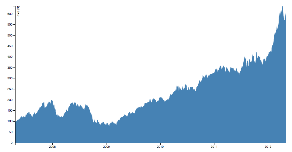
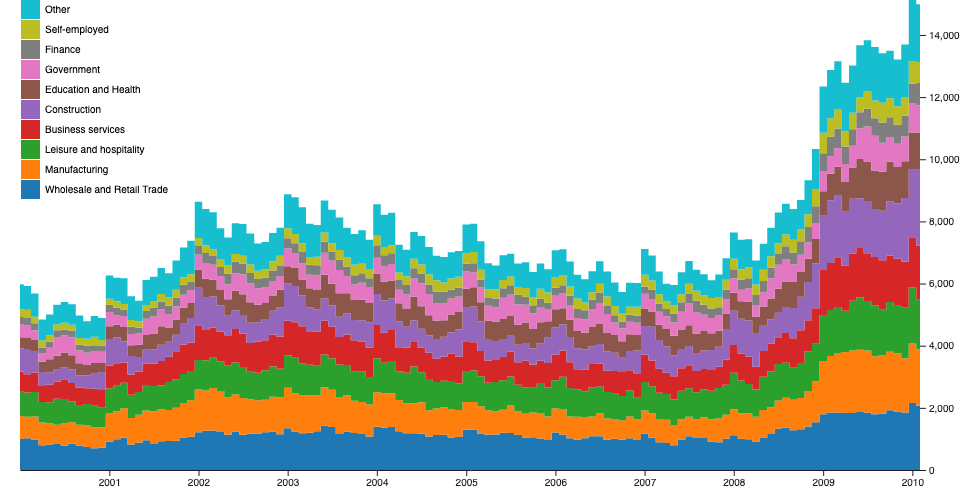
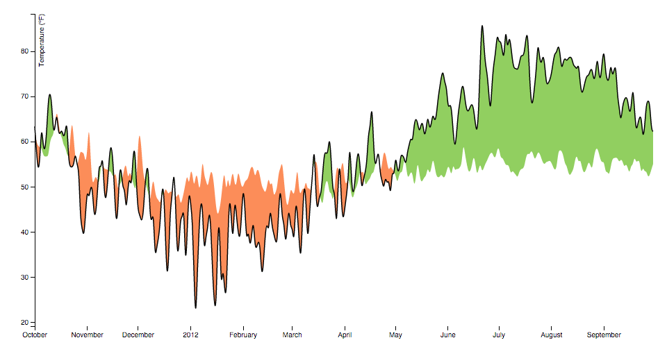
The area generator produces an area, as in an area chart. An area is defined by two bounding lines, either splines or polylines. Typically, the two lines share the same x-values (x0 = x1), differing only in y-value (y0 and y1); most commonly, y0 is defined as a constant representing zero. The first line (the topline) is defined by x1 and y1 and is rendered first; the second line (the baseline) is defined by x0 and y0 and is rendered second, with the points in reverse order. With a linear curve, this produces a clockwise polygon.

# area()

Constructs a new area generator with the default settings.

# area(data)

Generates an area for the given array of data. Depending on this area generator’s associated curve, the given input data may need to be sorted by x-value before being passed to the area generator. If the area generator has a context, then the area is rendered to this context as a sequence of path method calls and this function returns void. Otherwise, a path data string is returned.

# area.x([x])

If x is specified, sets x0 to x and x1 to null and returns this area generator. If x is not specified, returns the current x0 accessor.

# area.x0([x])

If x is specified, sets the x0 accessor to the specified function or number and returns this area generator. If x is not specified, returns the current x0 accessor, which defaults to:

function x(d) {
  return d[0];
}

When an area is generated, the x0 accessor will be invoked for each defined element in the input data array, being passed the element d, the index i, and the array data as three arguments. The default x0 accessor assumes that the input data are two-element arrays of numbers. If your data are in a different format, or if you wish to transform the data before rendering, then you should specify a custom accessor. For example, if x is a time scale and y is a linear scale:

var data = [
  {date: new Date(2007, 3, 24), value: 93.24},
  {date: new Date(2007, 3, 25), value: 95.35},
  {date: new Date(2007, 3, 26), value: 98.84},
  {date: new Date(2007, 3, 27), value: 99.92},
  {date: new Date(2007, 3, 30), value: 99.80},
  {date: new Date(2007, 4,  1), value: 99.47},
  …
];

var a = area()
    .x(function(d) { return x(d.date); })
    .y1(function(d) { return y(d.value); })
    .y0(y(0));

# area.x1([x])

If x is specified, sets the x1 accessor to the specified function or number and returns this area generator. If x is not specified, returns the current x1 accessor, which defaults to null, indicating that the previously-computed x0 value should be reused for the x1 value.

When an area is generated, the x1 accessor will be invoked for each defined element in the input data array, being passed the element d, the index i, and the array data as three arguments. See area.x0 for more information.

# area.y([y])

If y is specified, sets y0 to y and y1 to null and returns this area generator. If y is not specified, returns the current y0 accessor.

# area.y0([y])

If y is specified, sets the y0 accessor to the specified function or number and returns this area generator. If y is not specified, returns the current y0 accessor, which defaults to:

function y() {
  return 0;
}

When an area is generated, the y0 accessor will be invoked for each defined element in the input data array, being passed the element d, the index i, and the array data as three arguments. See area.x0 for more information.

# area.y1([y])

If y is specified, sets the y1 accessor to the specified function or number and returns this area generator. If y is not specified, returns the current y1 accessor, which defaults to:

function y(d) {
  return d[1];
}

A null accessor is also allowed, indicating that the previously-computed y0 value should be reused for the y1 value. When an area is generated, the y1 accessor will be invoked for each defined element in the input data array, being passed the element d, the index i, and the array data as three arguments. See area.x0 for more information.

# area.defined([defined])

If defined is specified, sets the defined accessor to the specified function or boolean and returns this area generator. If defined is not specified, returns the current defined accessor, which defaults to:

function defined() {
  return true;
}

The default accessor thus assumes that the input data is always defined. When an area is generated, the defined accessor will be invoked for each element in the input data array, being passed the element d, the index i, and the array data as three arguments. If the given element is defined (i.e., if the defined accessor returns a truthy value for this element), the x0, x1, y0 and y1 accessors will subsequently be evaluated and the point will be added to the current area segment. Otherwise, the element will be skipped, the current area segment will be ended, and a new area segment will be generated for the next defined point. As a result, the generated area may have several discrete segments. For example:

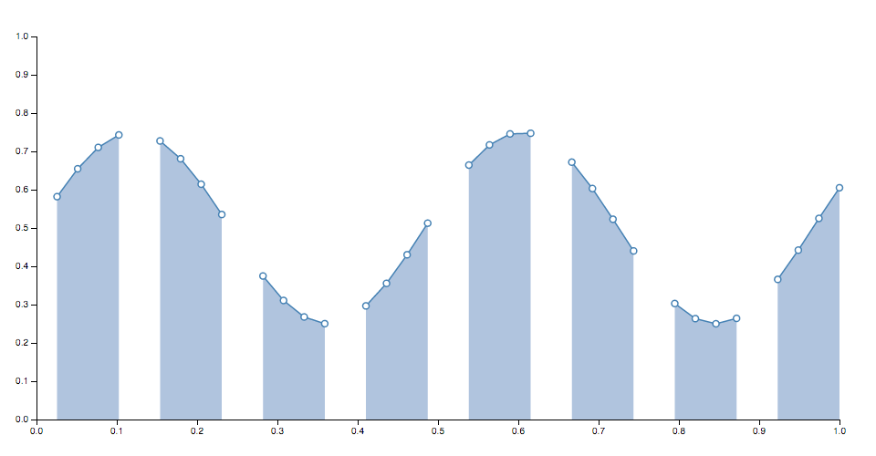
Note that if an area segment consists of only a single point, it may appear invisible unless rendered with rounded or square line caps. In addition, some curves such as cardinalOpen only render a visible segment if it contains multiple points.

# area.curve([curve[, parameters…]])

If curve is specified, sets the curve factory and returns this area generator. Any optional parameters, if specified, will be bound to the specified curve. If curve is not specified, returns the current curve factory, which defaults to linear.

# area.context([context])

If context is specified, sets the context and returns this area generator. If context is not specified, returns the current context, which defaults to null. If the context is not null, then the generated area is rendered to this context as a sequence of path method calls. Otherwise, a path data string representing the generated area is returned.

# radialArea()

Constructs a new radial area generator with the default settings. A radial area generator is equivalent to the standard Cartesian area generator, except the x and y accessors are replaced with angle and radius accessors. Radial areas are always positioned relative to ⟨0,0⟩; use a transform (see: SVG, Canvas) to change the origin.

# radialArea.angle([angle])

Equivalent to area.x, except the accessor returns the angle in radians, with 0 at -y (12 o’clock).

# radialArea.startAngle([angle])

Equivalent to area.x0, except the accessor returns the angle in radians, with 0 at -y (12 o’clock). Note: typically angle is used instead of setting separate start and end angles.

# radialArea.endAngle([angle])

Equivalent to area.x1, except the accessor returns the angle in radians, with 0 at -y (12 o’clock). Note: typically angle is used instead of setting separate start and end angles.

# radialArea.radius([radius])

Equivalent to area.y, except the accessor returns the radius: the distance from the origin ⟨0,0⟩.

# radialArea.innerRadius([radius])

Equivalent to area.y0, except the accessor returns the radius: the distance from the origin ⟨0,0⟩.

# radialArea.outerRadius([radius])

Equivalent to area.y1, except the accessor returns the radius: the distance from the origin ⟨0,0⟩.

# radialArea.defined([defined])

Equivalent to area.defined.

# radialArea.curve([curve[, parameters…]])

Equivalent to area.curve. Note that the monotone curve is not recommended for radial areas because it assumes that the data is monotonic in x, which is typically untrue of radial areas.

# radialArea.context([context])

Equivalent to line.context.

Curves

While lines are defined as a sequence of two-dimensional [x, y] points, and areas are similarly defined by a topline and a baseline, there remains the task of transforming this discrete representation into a continuous shape: i.e., how to interpolate between the points. A variety of curves are provided for this purpose.

Curves are typically not constructed or used directly, instead being passed to line.curve and area.curve.

# basis(context)

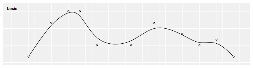
Produces a cubic basis spline using the specified control points. The first and last points are triplicated such that the spline starts at the first point and ends at the last point, and is tangent to the line between the first and second points, and to the line between the penultimate and last points.

# basisClosed(context)

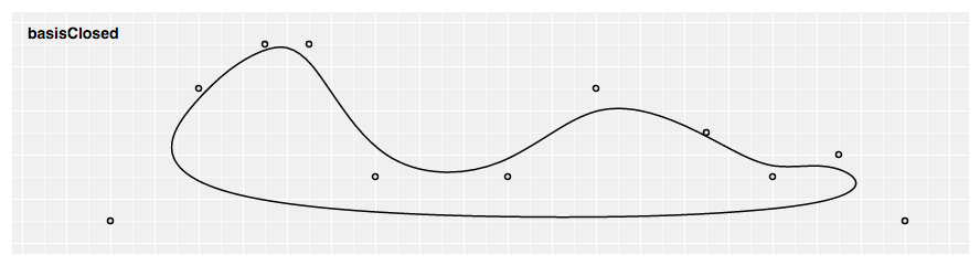
Produces a closed cubic basis spline using the specified control points. When a line segment ends, the first three control points are repeated, producing a closed loop with C2 continuity.

# basisOpen(context)

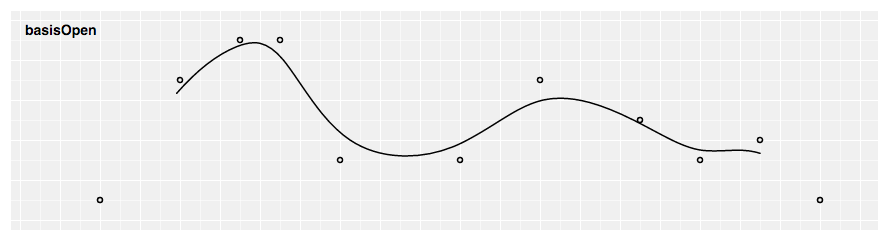
Produces a cubic basis spline using the specified control points. Unlike basis, the first and last points are not repeated, and thus the curve typically does not intersect these points.

# bundle(context[, beta])

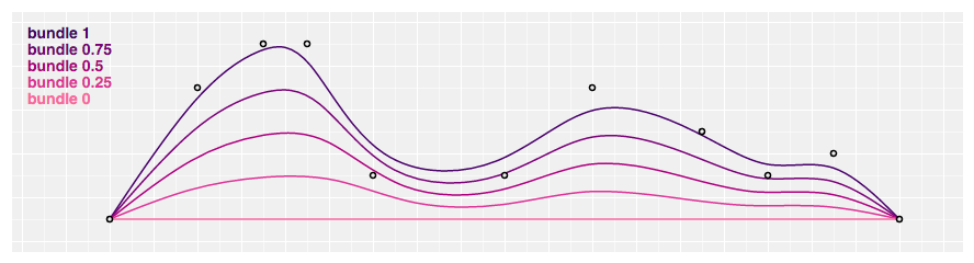
Produces a straighted cubic basis spline using the specified control points, with the spline straightened according to the specified parameter beta in the range [0, 1]. If beta equals zero, a straight line between the first and last point is produced; if beta equals one, a standard basis spline is produced. If beta is not specified, it defaults to 0.85. This curve is typically used in hierarchical edge bundling to disambiguate connections, as proposed by Danny Holten in Hierarchical Edge Bundles: Visualization of Adjacency Relations in Hierarchical Data; beta represents the bundle strength.

# cardinal(context[, tension])

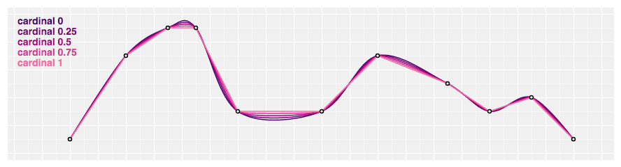
Produces a cubic cardinal spline using the specified control points, with one-sided differences used for the first and last piece. The tension parameter in the range [0, 1] determines the length of the tangents: a tension of one yields all zero tangents, equivalent to linear; a tension of zero produces a uniform Catmull–Rom spline. If tension is not specified, it defaults to zero.

# cardinalClosed(context[, tension])

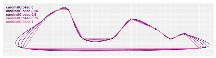
Produces a closed cubic cardinal spline using the specified control points. When a line segment ends, the first three control points are repeated, producing a closed loop. The tension parameter in the range [0, 1] determines the length of the tangents: a tension of one yields all zero tangents, equivalent to linearClosed; a tension of zero produces a closed uniform Catmull–Rom spline.

# cardinalOpen(context[, tension])

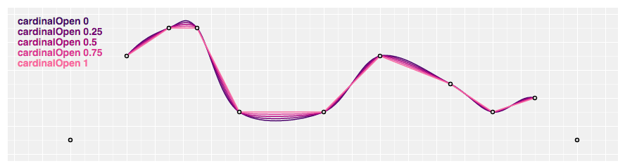
Produces a cubic cardinal spline using the specified control points. Unlike cardinal, one-sided differences are not used for the first and last piece, and thus the curve starts at the second point and ends at the penultimate point.

# catmullRom(context[, alpha])

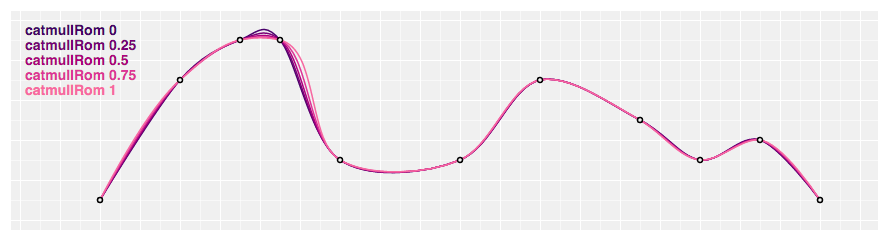
Produces a cubic Catmull–Rom spline using the specified control points and the parameter alpha, as proposed by Yuksel et al. in On the Parameterization of Catmull–Rom Curves, with one-sided differences used for the first and last piece. If alpha is zero, produces a uniform spline, equivalent to cardinal with a tension of zero; if alpha is one, produces a chordal spline; if alpha is 0.5, produces a centripetal spline. If alpha is not specified, it defaults to 0.5. Centripetal splines are recommended to avoid self-intersections and overshoot.

# catmullRomClosed(context[, alpha])

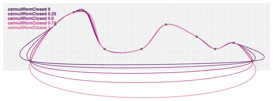
Produces a closed cubic Catmull–Rom spline using the specified control points and the parameter alpha, as proposed by Yuksel et al. When a line segment ends, the first three control points are repeated, producing a closed loop. If alpha is zero, produces a uniform spline, equivalent to cardinalClosed with a tension of zero; if alpha is one, produces a chordal spline; if alpha is 0.5, produces a centripetal spline. If alpha is not specified, it defaults to 0.5. Centripetal splines are recommended to avoid self-intersections and overshoot.

# catmullRomOpen(context[, alpha])

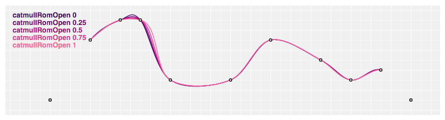
Produces a cubic Catmull–Rom spline using the specified control points and the parameter alpha, as proposed by Yuksel et al. Unlike catmullRom, one-sided differences are not used for the first and last piece, and thus the curve starts at the second point and ends at the penultimate point. If alpha is zero, produces a uniform spline, equivalent to cardinalOpen with a tension of zero; if alpha is one, produces a chordal spline; if alpha is 0.5, produces a centripetal spline. If alpha is not specified, it defaults to 0.5. Centripetal splines are recommended to avoid self-intersections and overshoot.

# linear(context)

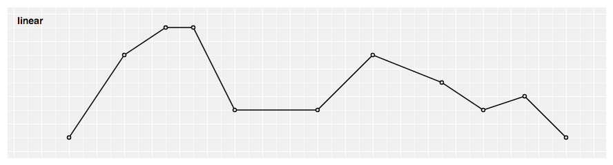
Produces a polyline through the specified points.

# linearClosed(context)

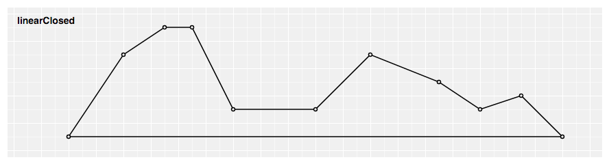
Produces a closed polyline through the specified points by repeating the first point when the line segment ends.

# monotone(context)

Produces a cubic spline that preserves monotonicity in y, as proposed by Steffen in A simple method for monotonic interpolation in one dimension: “a smooth curve with continuous first-order derivatives that passes through any given set of data points without spurious oscillations. Local extrema can occur only at grid points where they are given by the data, but not in between two adjacent grid points.” Assumes that the input data is monotonic in x.

# natural(context)

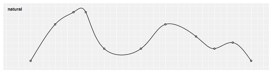
Produces a natural cubic spline with the second derivative of the spline set to zero at the endpoints.

# step(context)

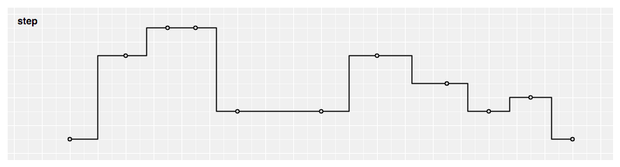
Produces a piecewise constant function (a step function) consisting of alternating horizontal and vertical lines. The y-value changes at the midpoint of each pair of adjacent x-values.

# stepAfter(context)

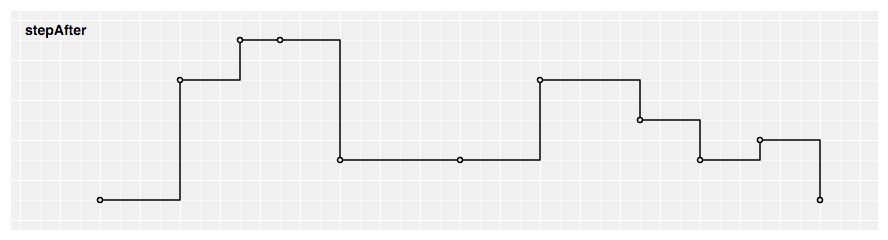
Produces a piecewise constant function (a step function) consisting of alternating horizontal and vertical lines. The y-value changes after the x-value.

# stepBefore(context)

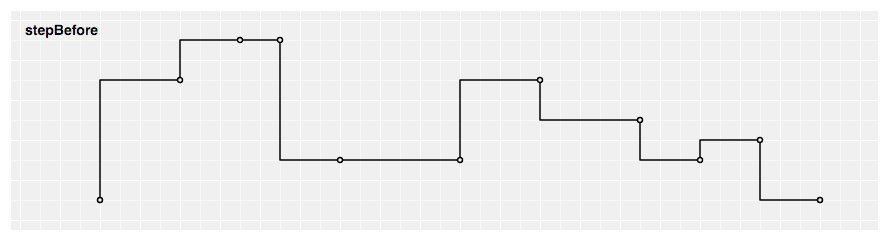
Produces a piecewise constant function (a step function) consisting of alternating horizontal and vertical lines. The y-value changes before the x-value.

Custom Curves

Curves are typically not used directly, instead being passed to line.curve and area.curve. However, you can define your own curve implementation should none of the built-in curves satisfy your needs using the following interface. You can also use this low-level interface with a built-in curve type as an alternative to the line and area generators.

# curve.areaStart()

Indicates the start of a new area segment. Each area segment consists of exactly two line segments: the topline, followed by the baseline, with the baseline points in reverse order.

# curve.areaEnd()

Indicates the end of the current area segment.

# curve.lineStart()

Indicates the start of a new line segment. Zero or more points will follow.

# curve.lineEnd()

Indicates the end of the current line segment.

# curve.point(x, y)

Indicates a new point in the current line segment with the given x- and y-values.

Symbols

Symbols provide a categorical shape encoding as is commonly used in scatterplots. Symbols are always centered at ⟨0,0⟩; use a transform (see: SVG, Canvas) to move the arc to a different position.

# symbol()

Constructs a new symbol generator with the default settings.

# symbol(arguments…)

Generates a symbol for the given arguments. The arguments are arbitrary; they are simply propagated to the symbol generator’s accessor functions along with the this object. For example, with the default settings, no arguments are needed to produce a circle with area 64 square pixels. If the symbol generator has a context, then the symbol is rendered to this context as a sequence of path method calls and this function returns void. Otherwise, a path data string is returned.

# symbol.type([type])

If type is specified, sets the symbol type and returns this line generator. If type is not specified, returns the current symbol type, which defaults to circle. See symbols for the set of built-in symbol types.

# symbol.size([size])

If size is specified, sets the size to the specified function or number and returns this symbol generator. If size is not specified, returns the current size accessor, which defaults to:

function size() {
  return 64;
}

Specifying the size as a function is useful for constructing a scatterplot with a size encoding. If you wish to scale the symbol to fit a given bounding box, rather than by area, try SVG’s getBBox.

# symbol.context([context])

If context is specified, sets the context and returns this symbol generator. If context is not specified, returns the current context, which defaults to null. If the context is not null, then the generated symbol is rendered to this context as a sequence of path method calls. Otherwise, a path data string representing the generated symbol is returned.

# symbols

An array containing the set of all built-in symbol types: circle, cross, diamond, square, down-pointing triangle, and up-pointing triangle. Useful for constructing the range of an ordinal scale should you wish to use a shape encoding for categorical data.

# circle

A circle.

# cross

A Greek cross with arms of equal length.

# diamond

A rhombus.

# square

A square.

# triangleDown

A down-pointing triangle.

# triangleUp

An up-pointing triangle.

Custom Symbol Types

Symbol types are typically not used directly, instead being passed to symbol.type. However, you can define your own sumbol type implementation should none of the built-in types satisfy your needs using the following interface. You can also use this low-level interface with a built-in symbol type as an alternative to the symbol generator.

# symbolType.draw(context, size)

Renders this symbol type to the specified context with the specified size in square pixels. The context implements the CanvasPathMethods interface. (Note that this is a subset of the CanvasRenderingContext2D interface!)

Changes from D3 3.x:

• You can now render shapes to Canvas by specifying a context (e.g., line.context)! See d3-path for how it works.

• The interpretation of the cardinal spline tension parameter has been fixed. The default cardinal tension is now 0 (corresponding to a uniform Catmull–Rom spline), not 0.7. Due to a bug in 3.x, the tension parameter was previously only valid in the range [2/3, 1]; this corresponds to the new corrected range of [0, 1]. Thus, the new default value of 0 is equivalent to the old value of 2/3, and the default behavior is only slightly changed.

• To specify a cardinal spline tension of t, use line.curve(cardinal, t) instead of line.interpolate("cardinal").tension(t).

• To specify a custom line or area interpolator, implement a curve.

• Added natural cubic splines.

• Added Catmull–Rom splines, parameterized by alpha. If α = 0, produces a uniform Catmull–Rom spline equivalent to a Cardinal spline with zero tension; if α = 0.5, produces a centripetal spline; if α = 1.0, produces a chordal spline.

• By setting area.x1 or area.y1 to null, you can reuse the area.x0 or area.y0 value, rather than computing it twice. This is useful for nondeterministic values (e.g., jitter).

• Accessor functions now always return functions, even if the value was set to a constant.