Genetics algorithms draw direct inspiration from nature and seek to unlock the computational power of DNA. The rationale goes that if selective reproduction, natural selection, and random mutation could be responsible for the complexity of life on this planet, surely we can harness these principles to solve (or more accurately, approximate) NP-complete problems in polynomial time.
[Start] Generate random population of n chromosomes (suitable solutions for the problem
[Fitness] Evaluate the fitness f(x) of each chromosome x in the population
[Test] If the end condition is satisfied, stop and return the population. If not, generate a new population.
[New population] Create a new population by repeating following steps until the new population is complete:
    [Selection] Select two parent chromosomes from a population according to their fitness (the better fitness, the bigger chance to be selected)
    [Crossover] With a crossover probability cross over the parents to form a new offspring (children). If no crossover was performed, offspring is an exact copy of parents.
    [Mutation] With a mutation probability mutate new offspring at each locus (position in chromosome).
    [Accepting] Place new offspring in a new population
[Replace] Use new generated population for a further run of algorithm
[Loop] Go to the Fitness step
Chromosomes express a potential certificate through an encoding such as binary, values, or trees. For the 0-1 knapsack problem, we will use a binary array to express which items of the knapsack will be added (1's) and which will be omitted (0's).
We generate an initial population by creating random arrays of 1's and 0's. The population size is specified by the user. A larger population size will slow down the algorithm but allow for more genetic diversity. Larger populations, however, are usually faster at converging to a solution and less susceptible to local maximums. I decided upon a population size of 100 chromosomes after some experimentation. As you will find out later, there is no necessarily “right” configuration of variables such as population size, mutation rate, or maximum generations, just certain combinations that achieve better results.
This step evaluates how “fit” each chromosome is in relation to the specific problem. For the 0-1 knapsack, the chromosomes are each ranked by the total weight of the knapsack. If the weight of a specific chromosome is higher than the maximum weight, a random 1-value is altered and the chromosome is reevaluated until it doesn't exceed the maximum. The fitness of each chromosome in the population is stored in an array. An interesting note is that the fitness function takes advantage of the NP-complete-ness of the knapsack problem, that is, a certificate is checkable in polynomial time.
A new population (also called a generation) is created by “mating” the fittest chromosomes of the population.
The chromosomes are selected in a manner that those with a higher fitness are more likely to be selected as mates. The type of selection that I implemented is called roulette-wheel selection, though other methods of selection such as rank selection, group selection, and steady state selection exist. Roulette-wheel selection picks a random number between 0 and the sum of the fitnesses. Then, iterating through the fitness array, I subtract each individual fitness from my random number until the number is greater than or equal to zero. Whatever chromosome I stop on is selected to mate. Unlike in nature, we can use a tactic called elitism, and copy the fittest chromosome automatically from the population to the new generation. Elitism is an essential practice to ensure that we converge on an answer.
The crossover is analogous to biological “mating” of species. Our virtual chromosomes, however, are not double helices but a single strands of binary. The crossover function takes two “parents” and creates a new chromosome by splicing parts of one with parts of another. These are two examples of crossover types:
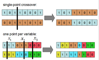
I used single point crossover for my implementation. For each set of parents a random pivot point is chosen and the bits up to that pivot point are exchanged, creating two new child chromosomes. I also chose to do 100% crossover for simplicity (aside from the elite chromosome). Some genetic algorithms with 85% crossover, for example, will copy 15% of the old population to the new population.
The mutation function, like random mutations in nature, keeps our populations genetically diverse. In our algorithm, mutations keep our succession of generations from converging at a local maximum. The mutation function goes through every bit of the new chromosomes and calculates whether to flip the bit based on a small probability.
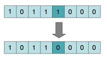
I chose a 1% probability for mutation based on experimentation. Having too large a mutation probability will cause the generations to be genetically unstable, and it will take longer to converge on a solution. (Remember that 100% mutation is essentially generating a random chromosome.) Too low of a mutation rate will keep the population locked in the genetic possibilities of the first generation.
After being generated, the new population replaces the old population. The fitness of the population is calculated then tested to see if an end condition is satisfied. In my algorithm I tested for a convergence factor of 90% or a maximum number of generations reached. I found that increasing the max number of generations proportional to ten times the input size helped scale the algorithm to larger inputs. If the end condition is not reached, the algorithm continues to loop, generating a new population and testing again.
Because I specified the maximum number of generations, the complexity of my program has an polynomial O(n^2) upper bound. Generating the initial population takes O(n). Both the crossover and mutation functions iterate over each chromosome once, taking O(n) time multiplied by the constant of the population size. Therefore the the loop takes O(n) time. This loop will run a maximum of 10*n times, making the total complexity of my algorithm O(n^2). This aligns with my experimentation on the running time. I ran 10 trials, with n = 10, 20, ... 100. Each trial consisted of 10 sets of randomly generated inputs of size n, and input was then tested 10 times. An average of the running time was taking over the 10 repetitions of the 10 sets for each trial. The average deviation and percent deviation of the solutions was also calculated for each set.
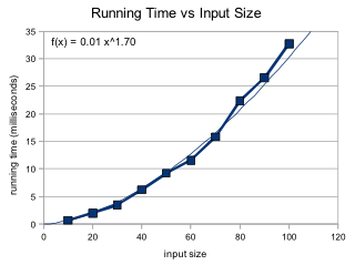
As we can see, the running time exhibits a power curve. The best fit power curve calculates an approximate actual running time of n1.7 which is within our O(n^2) bound.
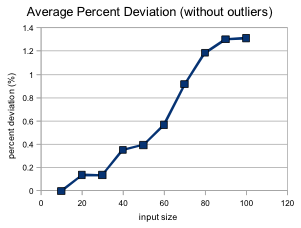
Because our genetic 0-1 knapsack algorithm is an approximation, an important thing to note is the average deviation of the generated solutions at different input sizes.
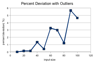
I found that whenever the maximum weight for the knapsack was very small (with a solution of mostly 0's) the average deviation could be up to 42%. This is most likely due to the way all chromosomes are altered so that they fit under the maximum weight before the new population is generated. One potential way to tackle this in the future would be to allow for chromosome with above-maximum weights to exist in the population, but with just a higher fitness penalty for exceeding the limit. After removing the obvious outliers, our percent deviation is as follows:
Sometimes we don't need THE best solution but a near best-solution. Many NP-complete problems, such as 0-1 knapsack program, can be approximated by simulating the computational power of evolution the natural world. Genetic algorithms themselves are very adaptable to the needs of the user, with many variables such as population size, convergence factor, maximum generations, mutation rate, and crossover ratio that can be altered for better results. There are also different ways of implementing the underlying structure of the algorithms, such as the chromosome encoding or selection factor. Further experiments could seek to explore the different combinations of such options on the 0-1 knapsack or other NP-complete problems.
- “Solving the 0-1 Knapsack Problem with Genetic Algorithms” by Maya Hristakev and Dipti Shresth.
- “Introduction to Genetic Algorithms” (Basic Structure of a Genetic Algorithm attributed to this site.)
- Dylan Estep's STARS presentation from junior year in high school. (All diagrams attributed to this presentation.)

