chrisyang/lstm-human-activity-recognition

Human activity recognition using TensorFlow on smartphone sensors dataset and an LSTM RNN. Classifying the type of movement amongst six categories (WALKING, WALKING_UPSTAIRS, WALKING_DOWNSTAIRS, SITTING, STANDING, LAYING).

LSTM for Human Activity Recognition

Human activity recognition using smartphones dataset and an LSTM RNN. Classifying the type of movement amongst six categories:

• WALKING,
• WALKING_UPSTAIRS,
• WALKING_DOWNSTAIRS,
• SITTING,
• STANDING,
• LAYING.

Video dataset overview

Follow this link to see a video of the 6 activities recorded in the experiment with one of the participants:

[Watch video]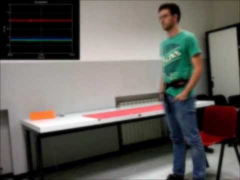

Details about input data

I will be using an LSTM on the data to learn (as a cellphone attached on the waist) to recognise the type of activity that the user is doing. The dataset's description goes like this:

The sensor signals (accelerometer and gyroscope) were pre-processed by applying noise filters and then sampled in fixed-width sliding windows of 2.56 sec and 50% overlap (128 readings/window). The sensor acceleration signal, which has gravitational and body motion components, was separated using a Butterworth low-pass filter into body acceleration and gravity. The gravitational force is assumed to have only low frequency components, therefore a filter with 0.3 Hz cutoff frequency was used.

That said, I will use the almost raw data: only the gravity effect has been filtered out of the accelerometer as a preprocessing step for another 3D feature as an input to help learning.

What is an RNN?

As explained in this article, an RNN takes many input vectors to process them and output other vectors. It can be roughly pictured like in the image below, imagining each rectangle has a vectorial depth and other special hidden quirks in the image below. In our case, the "many to one" architecture is used: we accept time series of feature vectors (one vector per time step) to convert them to a probability vector at the output for classification. Note that a "one to one" architecture would be a standard feedforward neural network.

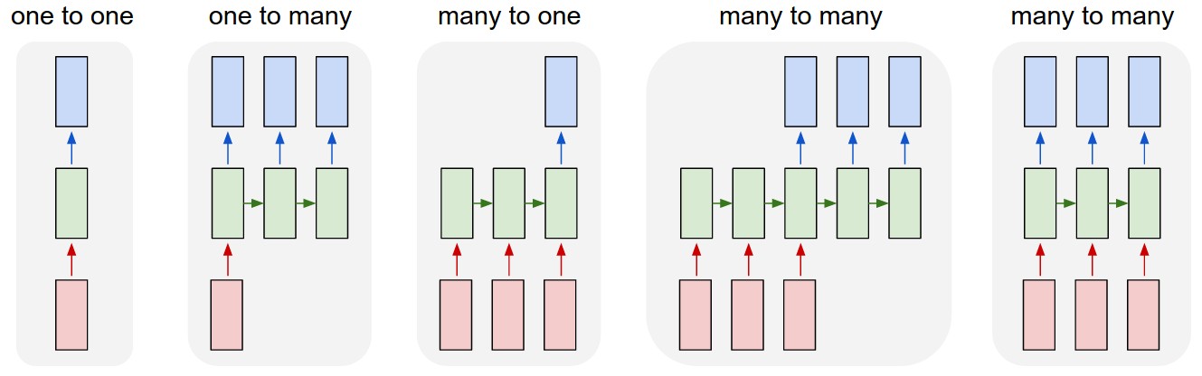
An LSTM is an improved RNN. It is more complex, but easier to train, avoiding what is called the vanishing gradient problem and the exploding gradient problem.

Results

Scroll on! Nice visuals awaits.

# All Includes

import numpy as np
import matplotlib
import matplotlib.pyplot as plt
import tensorflow as tf  # Version r0.10
from sklearn import metrics

import os

# Useful Constants

# Those are separate normalised input features for the neural network
INPUT_SIGNAL_TYPES = [
    "body_acc_x_",
    "body_acc_y_",
    "body_acc_z_",
    "body_gyro_x_",
    "body_gyro_y_",
    "body_gyro_z_",
    "total_acc_x_",
    "total_acc_y_",
    "total_acc_z_"
]

# Output classes to learn how to classify
LABELS = [
    "WALKING", 
    "WALKING_UPSTAIRS", 
    "WALKING_DOWNSTAIRS", 
    "SITTING", 
    "STANDING", 
    "LAYING"
] 

Let's start by downloading the data:

# Note: Linux bash commands start with a "!" inside those "ipython notebook" cells

DATA_PATH = "data/"

!pwd && ls
os.chdir(DATA_PATH)
!pwd && ls

!python download_dataset.py

!pwd && ls
os.chdir("..")
!pwd && ls

DATASET_PATH = DATA_PATH + "UCI HAR Dataset/"
print("\n" + "Dataset is now located at: " + DATASET_PATH)

/home/gui/Documents/GIT/LSTM-Human-Activity-Recognition
data  LICENSE  LSTM_files  LSTM.ipynb  lstm.py	README.md
/home/gui/Documents/GIT/LSTM-Human-Activity-Recognition/data
download_dataset.py  __MACOSX  source.txt  UCI HAR Dataset  UCI HAR Dataset.zip

Downloading...
Dataset already downloaded. Did not download twice.

Extracting...
Dataset already extracted. Did not extract twice.

/home/gui/Documents/GIT/LSTM-Human-Activity-Recognition/data
download_dataset.py  __MACOSX  source.txt  UCI HAR Dataset  UCI HAR Dataset.zip
/home/gui/Documents/GIT/LSTM-Human-Activity-Recognition
data  LICENSE  LSTM_files  LSTM.ipynb  lstm.py	README.md

Dataset is now located at: data/UCI HAR Dataset/

Preparing dataset:

TRAIN = "train/"
TEST = "test/"


# Load "X" (the neural network's training and testing inputs)

def load_X(X_signals_paths):
    X_signals = []
    
    for signal_type_path in X_signals_paths:
        file = open(signal_type_path, 'rb')
        # Read dataset from disk, dealing with text files' syntax
        X_signals.append(
            [np.array(serie, dtype=np.float32) for serie in [
                row.replace('  ', ' ').strip().split(' ') for row in file
            ]]
        )
        file.close()
    
    return np.transpose(np.array(X_signals), (1, 2, 0))

X_train_signals_paths = [
    DATASET_PATH + TRAIN + "Inertial Signals/" + signal + "train.txt" for signal in INPUT_SIGNAL_TYPES
]
X_test_signals_paths = [
    DATASET_PATH + TEST + "Inertial Signals/" + signal + "test.txt" for signal in INPUT_SIGNAL_TYPES
]

X_train = load_X(X_train_signals_paths)
X_test = load_X(X_test_signals_paths)


# Load "y" (the neural network's training and testing outputs)

def load_y(y_path):
    file = open(y_path, 'rb')
    # Read dataset from disk, dealing with text file's syntax
    y_ = np.array(
        [elem for elem in [
            row.replace('  ', ' ').strip().split(' ') for row in file
        ]], 
        dtype=np.int32
    )
    file.close()
    
    # Substract 1 to each output class for friendly 0-based indexing 
    return y_ - 1

y_train_path = DATASET_PATH + TRAIN + "y_train.txt"
y_test_path = DATASET_PATH + TEST + "y_test.txt"

y_train = load_y(y_train_path)
y_test = load_y(y_test_path)

Additionnal Parameters:

Here are some core parameter definitions for the training.

The whole neural network's structure could be summarised by enumerating those parameters and the fact an LSTM is used.

# Input Data 

training_data_count = len(X_train)  # 7352 training series (with 50% overlap between each serie)
test_data_count = len(X_test)  # 2947 testing series
n_steps = len(X_train[0])  # 128 timesteps per series
n_input = len(X_train[0][0])  # 9 input parameters per timestep


# LSTM Neural Network's internal structure

n_hidden = 32 # Hidden layer num of features
n_classes = 6 # Total classes (should go up, or should go down)


# Training 

learning_rate = 0.0025
lambda_loss_amount = 0.0015
training_iters = training_data_count * 300  # Loop 300 times on the dataset
batch_size = 1500
display_iter = 30000  # To show test set accuracy during training


# Some debugging info

print "Some useful info to get an insight on dataset's shape and normalisation:"
print "(X shape, y shape, every X's mean, every X's standard deviation)"
print (X_test.shape, y_test.shape, np.mean(X_test), np.std(X_test))
print "The dataset is therefore properly normalised, as expected, but not yet one-hot encoded."

Some useful info to get an insight on dataset's shape and normalisation:
(X shape, y shape, every X's mean, every X's standard deviation)
((2947, 128, 9), (2947, 1), 0.099147044, 0.39534995)
The dataset is therefore properly normalised, as expected, but not yet one-hot encoded.

Utility functions for training:

def LSTM_RNN(_X, _weights, _biases):
    # Function returns a tensorflow LSTM (RNN) artificial neural network from given parameters. 
    # Moreover, two LSTM cells are stacked which adds deepness to the neural network. 
    # Note, some code of this notebook is inspired from an slightly different 
    # RNN architecture used on another dataset: 
    # https://tensorhub.com/aymericdamien/tensorflow-rnn

    # (NOTE: This step could be greatly optimised by shaping the dataset once
    # input shape: (batch_size, n_steps, n_input)
    _X = tf.transpose(_X, [1, 0, 2])  # permute n_steps and batch_size
    # Reshape to prepare input to hidden activation
    _X = tf.reshape(_X, [-1, n_input]) 
    # new shape: (n_steps*batch_size, n_input)
    
    # Linear activation
    _X = tf.nn.relu(tf.matmul(_X, _weights['hidden']) + _biases['hidden'])
    # Split data because rnn cell needs a list of inputs for the RNN inner loop
    _X = tf.split(0, n_steps, _X) 
    # new shape: n_steps * (batch_size, n_hidden)

    # Define two stacked LSTM cells (two recurrent layers deep) with tensorflow
    lstm_cell_1 = tf.nn.rnn_cell.BasicLSTMCell(n_hidden, forget_bias=1.0, state_is_tuple=True)
    lstm_cell_2 = tf.nn.rnn_cell.BasicLSTMCell(n_hidden, forget_bias=1.0, state_is_tuple=True)
    lstm_cells = tf.nn.rnn_cell.MultiRNNCell([lstm_cell_1, lstm_cell_2], state_is_tuple=True)
    # Get LSTM cell output
    outputs, states = tf.nn.rnn(lstm_cells, _X, dtype=tf.float32)

    # Get last time step's output feature for a "many to one" style classifier, 
    # as in the image describing RNNs at the top of this page
    lstm_last_output = outputs[-1]
    
    # Linear activation
    return tf.matmul(lstm_last_output, _weights['out']) + _biases['out']


def extract_batch_size(_train, step, batch_size):
    # Function to fetch a "batch_size" amount of data from "(X|y)_train" data. 
    
    shape = list(_train.shape)
    shape[0] = batch_size
    batch_s = np.empty(shape)

    for i in range(batch_size):
        # Loop index
        index = ((step-1)*batch_size + i) % len(_train)
        batch_s[i] = _train[index] 

    return batch_s


def one_hot(y_):
    # Function to encode output labels from number indexes 
    # e.g.: [[5], [0], [3]] --> [[0, 0, 0, 0, 0, 1], [1, 0, 0, 0, 0, 0], [0, 0, 0, 1, 0, 0]]
    
    y_ = y_.reshape(len(y_))
    n_values = np.max(y_) + 1
    return np.eye(n_values)[np.array(y_, dtype=np.int32)]  # Returns FLOATS

Let's get serious and build the neural network:

# Graph input/output
x = tf.placeholder(tf.float32, [None, n_steps, n_input])
y = tf.placeholder(tf.float32, [None, n_classes])

# Graph weights
weights = {
    'hidden': tf.Variable(tf.random_normal([n_input, n_hidden])), # Hidden layer weights
    'out': tf.Variable(tf.random_normal([n_hidden, n_classes], mean=1.0))
}
biases = {
    'hidden': tf.Variable(tf.random_normal([n_hidden])),
    'out': tf.Variable(tf.random_normal([n_classes]))
}

pred = LSTM_RNN(x, weights, biases)

# Loss, optimizer and evaluation
l2 = lambda_loss_amount * sum(
    tf.nn.l2_loss(tf_var) for tf_var in tf.trainable_variables()
) # L2 loss prevents this overkill neural network to overfit the data
cost = tf.reduce_mean(tf.nn.softmax_cross_entropy_with_logits(pred, y)) + l2 # Softmax loss
optimizer = tf.train.AdamOptimizer(learning_rate=learning_rate).minimize(cost) # Adam Optimizer

correct_pred = tf.equal(tf.argmax(pred,1), tf.argmax(y,1))
accuracy = tf.reduce_mean(tf.cast(correct_pred, tf.float32))

Hooray, now train the neural network:

# To keep track of training's performance
test_losses = []
test_accuracies = []
train_losses = []
train_accuracies = []

# Launch the graph
sess = tf.InteractiveSession(config=tf.ConfigProto(log_device_placement=True))
init = tf.initialize_all_variables()
sess.run(init)

# Perform Training steps with "batch_size" amount of example data at each loop
step = 1
while step * batch_size <= training_iters:
    batch_xs =         extract_batch_size(X_train, step, batch_size)
    batch_ys = one_hot(extract_batch_size(y_train, step, batch_size))

    # Fit training using batch data
    _, loss, acc = sess.run(
        [optimizer, cost, accuracy],
        feed_dict={
            x: batch_xs, 
            y: batch_ys
        }
    )
    train_losses.append(loss)
    train_accuracies.append(acc)
    
    # Evaluate network only at some steps for faster training: 
    if (step*batch_size % display_iter == 0) or (step == 1) or (step * batch_size > training_iters):
        
        # To not spam console, show training accuracy/loss in this "if"
        print "Training iter #" + str(step*batch_size) + \
              ":   Batch Loss = " + "{:.6f}".format(loss) + \
              ", Accuracy = {}".format(acc)
        
        # Evaluation on the test set (no learning made here - just evaluation for diagnosis)
        loss, acc = sess.run(
            [cost, accuracy], 
            feed_dict={
                x: X_test,
                y: one_hot(y_test)
            }
        )
        test_losses.append(loss)
        test_accuracies.append(acc)
        print "PERFORMANCE ON TEST SET: " + \
              "Batch Loss = {}".format(loss) + \
              ", Accuracy = {}".format(acc)

    step += 1

print "Optimization Finished!"

# Accuracy for test data

one_hot_predictions, accuracy, final_loss = sess.run(
    [pred, accuracy, cost],
    feed_dict={
        x: X_test,
        y: one_hot(y_test)
    }
)

test_losses.append(final_loss)
test_accuracies.append(accuracy)

print "FINAL RESULT: " + \
      "Batch Loss = {}".format(final_loss) + \
      ", Accuracy = {}".format(accuracy)

Training iter #1500:   Batch Loss = 3.074432, Accuracy = 0.100666671991
PERFORMANCE ON TEST SET: Batch Loss = 2.64702987671, Accuracy = 0.224635243416
Training iter #30000:   Batch Loss = 1.388876, Accuracy = 0.713999986649
PERFORMANCE ON TEST SET: Batch Loss = 1.42781305313, Accuracy = 0.678316831589
Training iter #60000:   Batch Loss = 1.243671, Accuracy = 0.755333304405
PERFORMANCE ON TEST SET: Batch Loss = 1.33201026917, Accuracy = 0.725822806358
Training iter #90000:   Batch Loss = 1.026985, Accuracy = 0.858666718006
PERFORMANCE ON TEST SET: Batch Loss = 1.29318606853, Accuracy = 0.784526586533
Training iter #120000:   Batch Loss = 0.950223, Accuracy = 0.88666665554
PERFORMANCE ON TEST SET: Batch Loss = 1.19165813923, Accuracy = 0.818459331989
Training iter #150000:   Batch Loss = 0.821248, Accuracy = 0.934666633606
PERFORMANCE ON TEST SET: Batch Loss = 1.1244571209, Accuracy = 0.840515732765
Training iter #180000:   Batch Loss = 0.852562, Accuracy = 0.895999968052
PERFORMANCE ON TEST SET: Batch Loss = 1.09874331951, Accuracy = 0.85985738039
Training iter #210000:   Batch Loss = 0.975475, Accuracy = 0.886000037193
PERFORMANCE ON TEST SET: Batch Loss = 1.00003457069, Accuracy = 0.87852036953
Training iter #240000:   Batch Loss = 0.778386, Accuracy = 0.943333387375
PERFORMANCE ON TEST SET: Batch Loss = 1.01710581779, Accuracy = 0.87852036953
Training iter #270000:   Batch Loss = 0.687293, Accuracy = 0.942666709423
PERFORMANCE ON TEST SET: Batch Loss = 0.985704541206, Accuracy = 0.885646343231
Training iter #300000:   Batch Loss = 0.648103, Accuracy = 0.974000036716
PERFORMANCE ON TEST SET: Batch Loss = 1.01484704018, Accuracy = 0.873769819736
Training iter #330000:   Batch Loss = 0.759852, Accuracy = 0.948000073433
PERFORMANCE ON TEST SET: Batch Loss = 0.960080265999, Accuracy = 0.871394515038
Training iter #360000:   Batch Loss = 0.739065, Accuracy = 0.923333406448
PERFORMANCE ON TEST SET: Batch Loss = 0.955386519432, Accuracy = 0.880556344986
Training iter #390000:   Batch Loss = 0.721678, Accuracy = 0.932666659355
PERFORMANCE ON TEST SET: Batch Loss = 0.999629855156, Accuracy = 0.860875368118
Training iter #420000:   Batch Loss = 0.629302, Accuracy = 0.953333437443
PERFORMANCE ON TEST SET: Batch Loss = 0.959317803383, Accuracy = 0.874109148979
Training iter #450000:   Batch Loss = 0.611473, Accuracy = 0.955333292484
PERFORMANCE ON TEST SET: Batch Loss = 0.913493096828, Accuracy = 0.884628295898
Training iter #480000:   Batch Loss = 0.610332, Accuracy = 0.942000031471
PERFORMANCE ON TEST SET: Batch Loss = 0.95140516758, Accuracy = 0.874109148979
Training iter #510000:   Batch Loss = 0.596108, Accuracy = 0.972666740417
PERFORMANCE ON TEST SET: Batch Loss = 0.912526726723, Accuracy = 0.87987780571
Training iter #540000:   Batch Loss = 0.644551, Accuracy = 0.932000041008
PERFORMANCE ON TEST SET: Batch Loss = 0.915139496326, Accuracy = 0.877841830254
Training iter #570000:   Batch Loss = 0.631275, Accuracy = 0.92933344841
PERFORMANCE ON TEST SET: Batch Loss = 0.892684578896, Accuracy = 0.878181099892
Training iter #600000:   Batch Loss = 0.616123, Accuracy = 0.933333277702
PERFORMANCE ON TEST SET: Batch Loss = 0.905649662018, Accuracy = 0.874109208584
Training iter #630000:   Batch Loss = 0.518553, Accuracy = 0.983333408833
PERFORMANCE ON TEST SET: Batch Loss = 0.877397477627, Accuracy = 0.872751891613
Training iter #660000:   Batch Loss = 0.517939, Accuracy = 0.971333324909
PERFORMANCE ON TEST SET: Batch Loss = 0.873089075089, Accuracy = 0.882931649685
Training iter #690000:   Batch Loss = 0.501185, Accuracy = 0.980666697025
PERFORMANCE ON TEST SET: Batch Loss = 0.880154192448, Accuracy = 0.873769879341
Training iter #720000:   Batch Loss = 0.554758, Accuracy = 0.951333403587
PERFORMANCE ON TEST SET: Batch Loss = 0.843538284302, Accuracy = 0.881574392319
Training iter #750000:   Batch Loss = 0.563906, Accuracy = 0.938666701317
PERFORMANCE ON TEST SET: Batch Loss = 0.896262228489, Accuracy = 0.867322564125
Training iter #780000:   Batch Loss = 0.464500, Accuracy = 0.967333436012
PERFORMANCE ON TEST SET: Batch Loss = 0.871921360493, Accuracy = 0.874787867069
Training iter #810000:   Batch Loss = 0.482101, Accuracy = 0.952000081539
PERFORMANCE ON TEST SET: Batch Loss = 0.856980860233, Accuracy = 0.87682390213
Training iter #840000:   Batch Loss = 0.505377, Accuracy = 0.938666701317
PERFORMANCE ON TEST SET: Batch Loss = 0.790416657925, Accuracy = 0.884628295898
Training iter #870000:   Batch Loss = 0.458924, Accuracy = 0.972000002861
PERFORMANCE ON TEST SET: Batch Loss = 0.793853282928, Accuracy = 0.879877686501
Training iter #900000:   Batch Loss = 0.418589, Accuracy = 0.984000086784
PERFORMANCE ON TEST SET: Batch Loss = 0.887957155704, Accuracy = 0.870376586914
Training iter #930000:   Batch Loss = 1.169172, Accuracy = 0.695999979973
PERFORMANCE ON TEST SET: Batch Loss = 0.910101830959, Accuracy = 0.783169269562
Training iter #960000:   Batch Loss = 0.606064, Accuracy = 0.891333341599
PERFORMANCE ON TEST SET: Batch Loss = 0.852943599224, Accuracy = 0.829317867756
Training iter #990000:   Batch Loss = 0.470464, Accuracy = 0.961333394051
PERFORMANCE ON TEST SET: Batch Loss = 0.724700808525, Accuracy = 0.865965306759
Training iter #1020000:   Batch Loss = 0.437445, Accuracy = 0.969333350658
PERFORMANCE ON TEST SET: Batch Loss = 0.706804692745, Accuracy = 0.897522866726
Training iter #1050000:   Batch Loss = 0.416014, Accuracy = 0.974000096321
PERFORMANCE ON TEST SET: Batch Loss = 0.682184875011, Accuracy = 0.903970062733
Training iter #1080000:   Batch Loss = 0.453880, Accuracy = 0.972000002861
PERFORMANCE ON TEST SET: Batch Loss = 0.672256708145, Accuracy = 0.907702565193
Training iter #1110000:   Batch Loss = 0.471102, Accuracy = 0.938666701317
PERFORMANCE ON TEST SET: Batch Loss = 0.727611303329, Accuracy = 0.895826101303
Training iter #1140000:   Batch Loss = 0.464602, Accuracy = 0.942666709423
PERFORMANCE ON TEST SET: Batch Loss = 0.7117882967, Accuracy = 0.892772197723
Training iter #1170000:   Batch Loss = 0.399398, Accuracy = 0.957333445549
PERFORMANCE ON TEST SET: Batch Loss = 0.662129640579, Accuracy = 0.894129574299
Training iter #1200000:   Batch Loss = 0.465797, Accuracy = 0.940666735172
PERFORMANCE ON TEST SET: Batch Loss = 0.679540455341, Accuracy = 0.884967684746
Training iter #1230000:   Batch Loss = 0.479665, Accuracy = 0.938666641712
PERFORMANCE ON TEST SET: Batch Loss = 0.683512926102, Accuracy = 0.881913661957
Training iter #1260000:   Batch Loss = 0.390101, Accuracy = 0.977333366871
PERFORMANCE ON TEST SET: Batch Loss = 0.628258824348, Accuracy = 0.901255488396
Training iter #1290000:   Batch Loss = 0.420251, Accuracy = 0.94000005722
PERFORMANCE ON TEST SET: Batch Loss = 0.648212552071, Accuracy = 0.899898052216
Training iter #1320000:   Batch Loss = 0.432608, Accuracy = 0.95066678524
PERFORMANCE ON TEST SET: Batch Loss = 0.610033810139, Accuracy = 0.904648661613
Training iter #1350000:   Batch Loss = 0.403986, Accuracy = 0.938666701317
PERFORMANCE ON TEST SET: Batch Loss = 0.70320302248, Accuracy = 0.886325001717
Training iter #1380000:   Batch Loss = 0.358220, Accuracy = 0.968666732311
PERFORMANCE ON TEST SET: Batch Loss = 0.613206148148, Accuracy = 0.898540854454
Training iter #1410000:   Batch Loss = 0.341404, Accuracy = 0.973999977112
PERFORMANCE ON TEST SET: Batch Loss = 0.648775041103, Accuracy = 0.886664271355
Training iter #1440000:   Batch Loss = 0.368336, Accuracy = 0.97000002861
PERFORMANCE ON TEST SET: Batch Loss = 0.598120570183, Accuracy = 0.905666589737
Training iter #1470000:   Batch Loss = 0.390903, Accuracy = 0.956666707993
PERFORMANCE ON TEST SET: Batch Loss = 0.66110599041, Accuracy = 0.889039635658
Training iter #1500000:   Batch Loss = 0.400978, Accuracy = 0.939333379269
PERFORMANCE ON TEST SET: Batch Loss = 0.724209189415, Accuracy = 0.880217075348
Training iter #1530000:   Batch Loss = 0.323776, Accuracy = 0.965999960899
PERFORMANCE ON TEST SET: Batch Loss = 0.634877681732, Accuracy = 0.894468903542
Training iter #1560000:   Batch Loss = 0.336838, Accuracy = 0.959333360195
PERFORMANCE ON TEST SET: Batch Loss = 0.655008435249, Accuracy = 0.879877746105
Training iter #1590000:   Batch Loss = 0.363266, Accuracy = 0.944666743279
PERFORMANCE ON TEST SET: Batch Loss = 0.632539153099, Accuracy = 0.894129574299
Training iter #1620000:   Batch Loss = 0.315511, Accuracy = 0.976666688919
PERFORMANCE ON TEST SET: Batch Loss = 0.684278428555, Accuracy = 0.887003660202
Training iter #1650000:   Batch Loss = 0.328709, Accuracy = 0.952000081539
PERFORMANCE ON TEST SET: Batch Loss = 0.639604568481, Accuracy = 0.90057682991
Training iter #1680000:   Batch Loss = 0.376681, Accuracy = 0.934000015259
PERFORMANCE ON TEST SET: Batch Loss = 0.628734171391, Accuracy = 0.890057504177
Training iter #1710000:   Batch Loss = 0.373600, Accuracy = 0.945999979973
PERFORMANCE ON TEST SET: Batch Loss = 0.588403463364, Accuracy = 0.905666649342
Training iter #1740000:   Batch Loss = 0.304719, Accuracy = 0.969333350658
PERFORMANCE ON TEST SET: Batch Loss = 0.807882368565, Accuracy = 0.86732262373
Training iter #1770000:   Batch Loss = 0.484144, Accuracy = 0.916666686535
PERFORMANCE ON TEST SET: Batch Loss = 0.787532448769, Accuracy = 0.833050489426
Training iter #1800000:   Batch Loss = 0.328061, Accuracy = 0.961333394051
PERFORMANCE ON TEST SET: Batch Loss = 0.552209913731, Accuracy = 0.890396952629
Training iter #1830000:   Batch Loss = 0.361723, Accuracy = 0.953333318233
PERFORMANCE ON TEST SET: Batch Loss = 0.49697381258, Accuracy = 0.909399271011
Training iter #1860000:   Batch Loss = 0.381517, Accuracy = 0.934666693211
PERFORMANCE ON TEST SET: Batch Loss = 0.513538181782, Accuracy = 0.919239759445
Training iter #1890000:   Batch Loss = 0.316621, Accuracy = 0.954666733742
PERFORMANCE ON TEST SET: Batch Loss = 0.512967705727, Accuracy = 0.912113904953
Training iter #1920000:   Batch Loss = 0.300370, Accuracy = 0.960000038147
PERFORMANCE ON TEST SET: Batch Loss = 0.529131948948, Accuracy = 0.902273356915
Training iter #1950000:   Batch Loss = 0.306562, Accuracy = 0.956666707993
PERFORMANCE ON TEST SET: Batch Loss = 0.530484378338, Accuracy = 0.909399271011
Training iter #1980000:   Batch Loss = 0.318665, Accuracy = 0.954666733742
PERFORMANCE ON TEST SET: Batch Loss = 0.521255552769, Accuracy = 0.916185855865
Training iter #2010000:   Batch Loss = 0.423832, Accuracy = 0.949333369732
PERFORMANCE ON TEST SET: Batch Loss = 0.508657217026, Accuracy = 0.910417318344
Training iter #2040000:   Batch Loss = 0.335710, Accuracy = 0.950000107288
PERFORMANCE ON TEST SET: Batch Loss = 0.591941297054, Accuracy = 0.885646283627
Training iter #2070000:   Batch Loss = 0.335933, Accuracy = 0.933333337307
PERFORMANCE ON TEST SET: Batch Loss = 0.495988607407, Accuracy = 0.906345367432
Training iter #2100000:   Batch Loss = 0.271547, Accuracy = 0.986000061035
PERFORMANCE ON TEST SET: Batch Loss = 0.500951290131, Accuracy = 0.908720612526
Training iter #2130000:   Batch Loss = 0.278299, Accuracy = 0.970666706562
PERFORMANCE ON TEST SET: Batch Loss = 0.508447647095, Accuracy = 0.91856110096
Training iter #2160000:   Batch Loss = 0.270260, Accuracy = 0.963999986649
PERFORMANCE ON TEST SET: Batch Loss = 0.505264401436, Accuracy = 0.919239759445
Training iter #2190000:   Batch Loss = 0.273257, Accuracy = 0.968666732311
PERFORMANCE ON TEST SET: Batch Loss = 0.504503488541, Accuracy = 0.914149820805
Optimization Finished!
FINAL RESULT: Batch Loss = 0.510438203812, Accuracy = 0.914149880409

Training is good, but having visual insight is even better:

Okay, let's plot this simply in the notebook for now.

# (Inline plots: )
%matplotlib inline

font = {
    'family' : 'Bitstream Vera Sans',
    'weight' : 'bold',
    'size'   : 18
}
matplotlib.rc('font', **font)

width = 12
height = 12
plt.figure(figsize=(width, height))

indep_train_axis = np.array(range(batch_size, (len(train_losses)+1)*batch_size, batch_size))
plt.plot(indep_train_axis, np.array(train_losses),     "b--", label="Train losses")
plt.plot(indep_train_axis, np.array(train_accuracies), "g--", label="Train accuracies")

indep_test_axis = np.array(range(batch_size, len(test_losses)*display_iter, display_iter)[:-1] + [training_iters])
plt.plot(indep_test_axis, np.array(test_losses),     "b-", label="Test losses")
plt.plot(indep_test_axis, np.array(test_accuracies), "g-", label="Test accuracies")

plt.title("Training session's progress over iterations")
plt.legend(loc='upper right', shadow=True)
plt.ylabel('Training Progress (Loss or Accuracy values)')
plt.xlabel('Training iteration')

plt.show()

And finally, the multi-class confusion matrix and metrics!

# Results

predictions = one_hot_predictions.argmax(1)

print "Testing Accuracy: {}%".format(100*accuracy)

print ""
print "Precision: {}%".format(100*metrics.precision_score(y_test, predictions, average="weighted"))
print "Recall: {}%".format(100*metrics.recall_score(y_test, predictions, average="weighted"))
print "f1_score: {}%".format(100*metrics.f1_score(y_test, predictions, average="weighted"))

print ""
print "Confusion Matrix:"
confusion_matrix = metrics.confusion_matrix(y_test, predictions)
print confusion_matrix
normalised_confusion_matrix = np.array(confusion_matrix, dtype=np.float32)/np.sum(confusion_matrix)*100

print ""
print "Confusion matrix (normalised to % of total test data):"
print normalised_confusion_matrix
print ("Note: training and testing data is not equally distributed amongst classes, "
       "so it is normal that more than a 6th of the data is correctly classifier in the last category.")

# Plot Results: 
width = 12
height = 12
plt.figure(figsize=(width, height))
plt.imshow(
    normalised_confusion_matrix, 
    interpolation='nearest', 
    cmap=plt.cm.rainbow
)
plt.title("Confusion matrix \n(normalised to % of total test data)")
plt.colorbar()
tick_marks = np.arange(n_classes)
plt.xticks(tick_marks, LABELS, rotation=90)
plt.yticks(tick_marks, LABELS)
plt.tight_layout()
plt.ylabel('True label')
plt.xlabel('Predicted label')
plt.show()

Testing Accuracy: 91.4149880409%

Precision: 91.5553217851%
Recall: 91.4149983034%
f1_score: 91.4338139477%

Confusion Matrix:
[[467  21   0   0   8   0]
 [  6 451  14   0   0   0]
 [  4   2 414   0   0   0]
 [  1   7   0 396  87   0]
 [  1   1   0  74 456   0]
 [  0  27   0   0   0 510]]

Confusion matrix (normalised to % of total test data):
[[ 15.84662342   0.71258909   0.           0.           0.2714625    0.        ]
 [  0.20359688  15.30369854   0.47505939   0.           0.           0.        ]
 [  0.13573125   0.06786563  14.04818439   0.           0.           0.        ]
 [  0.03393281   0.2375297    0.          13.43739319   2.95215464   0.        ]
 [  0.03393281   0.03393281   0.           2.51102829  15.47336292   0.        ]
 [  0.           0.91618598   0.           0.           0.          17.30573463]]
Note: training and testing data is not equally distributed amongst classes, so it is normal that more than a 6th of the data is correctly classifier in the last category.

sess.close()

Conclusion

Outstandingly, the accuracy is of 91%!

This means that the neural networks is almost always able to correctly identify the movement type! Remember, the phone is attached on the waist and each series to classify has just a 128 sample window of two internal sensors (a.k.a. 2.56 seconds at 50 FPS), so those predictions are extremely accurate.

I specially did not expect such good results for guessing between "WALKING" "WALKING_UPSTAIRS" and "WALKING_DOWNSTAIRS" as a cellphone. Thought, it is still possible to see a little cluster on the matrix between those 3 classes. This is great.

It is also possible to see that it was hard to do the difference between "SITTING" and "STANDING". Those are seemingly almost the same thing from the point of view of a device placed on the belly, according to how the dataset was gathered.

I also tried my code without the gyroscope, using only the two 3D accelerometer's features (and not changing the training hyperparameters), and got an accuracy of 87%.

Improvements

In another repo of mine, the accuracy is pushed up to 94% using a special deep bidirectional architecture, and this architecture is tested on another dataset. If you want to learn more about deep learning, I have built a list of ressources that I found to be useful here.

References

The dataset can be found on the UCI Machine Learning Repository.

Davide Anguita, Alessandro Ghio, Luca Oneto, Xavier Parra and Jorge L. Reyes-Ortiz. A Public Domain Dataset for Human Activity Recognition Using Smartphones. 21th European Symposium on Artificial Neural Networks, Computational Intelligence and Machine Learning, ESANN 2013. Bruges, Belgium 24-26 April 2013.

If you want to cite my work, you can point to the URL of the GitHub repository:

https://github.com/guillaume-chevalier/LSTM-Human-Activity-Recognition

Connect with me

• https://ca.linkedin.com/in/chevalierg
• https://twitter.com/guillaume_che
• https://github.com/guillaume-chevalier/

# Let's convert this notebook to a README as the GitHub project's title page:
!jupyter nbconvert --to markdown LSTM.ipynb
!mv LSTM.md README.md

[NbConvertApp] Converting notebook LSTM.ipynb to markdown
[NbConvertApp] Support files will be in LSTM_files/
[NbConvertApp] Making directory LSTM_files
[NbConvertApp] Making directory LSTM_files
[NbConvertApp] Writing 31631 bytes to LSTM.md