![]()


This software can generate colour-colour diagram, colour-magnitude diagram in various photometric systems, plotting cooling profiles from different models, and compute theoretical white dwarf luminosity functions based on the built-in or supplied models of (1) initial mass function, (2) total stellar evolution lifetime, (3) initial-final mass relation, and (4) white dwarf cooling time.
the core parts of this work are three-fold: the first and the backbone of this work is the formatters that handle the output models from various works in the format as they are downloaded. This will allow the software to be updated with the newer models easily in the future. The second core part is the photometric fitter that solves for the WD parameters based on the photometry, with or without distance and reddening. The last part is to generate white dwarf luminosity function in bolometric magnitudes or in any of the photometric systems availalbe from the atmosphere model.
When using the RBFInterpolator, we strongly encourage the use of scipy 1.9+ which provides a speed gain of O(100) times.
Documentation and more examples can be found at Read the Docs.
If you have made use of the WDPhotTools, we would appreciate if you can refernce the follow article and the software itself. The BibTex of the two items are::
@article{10.1093/rasti/rzac006,
    author = {Lam, M C and Yuen, K W and Green, M J and Li, W},
    title = "{WDPhotTools – a white dwarf photometric toolkit in Python}",
    journal = {RAS Techniques and Instruments},
    volume = {1},
    number = {1},
    pages = {81-98},
    year = {2022},
    month = {12},
    issn = {2752-8200},
    doi = {10.1093/rasti/rzac006},
    url = {https://doi.org/10.1093/rasti/rzac006},
    eprint = {https://academic.oup.com/rasti/article-pdf/1/1/81/48321979/rzac006.pdf},
}
and
@software{marco_c_lam_2022_6595029,
    author       = {Marco C Lam and
                    K Yuen},
    title        = {WDPhotTools – a white dwarf photometric toolkit in Python},
    month        = may,
    year         = 2022,
    publisher    = {Zenodo},
    doi          = {10.5281/zenodo.6595029},
    url          = {https://doi.org/10.5281/zenodo.6595029}
}The cooling models only include the modelling of the bolometric lumninosity, the synthetic photometry is not usually provided. We have included the synthetic colours computed by the Montreal group. By default, it maps the (logg, Mbol) to Gaia G band (DR3). The DA cooling tracks can be generated with
from WDPhotTools import plotter

plotter.plot_atmosphere_model(invert_yaxis=True)
or with finer control by using the interpolators
from matplotlib import pyplot as plt
import numpy as np

from WDPhotTools.atmosphere_model_reader import AtmosphereModelReader

atm = AtmosphereModelReader()

# Default passband is G3
G = atm.interp_am()
BP = atm.interp_am(dependent="G3_BP")
RP = atm.interp_am(dependent="G3_RP")

logg = np.arange(7.0, 9.5, 0.5)
Mbol = np.arange(0.0, 20.0, 0.1)

plt.figure(1, figsize=(8, 8))
for i in logg:
    plt.plot(
        BP(i, Mbol) - RP(i, Mbol),
        G(i, Mbol),
        label=r"$\log(g) = {}$".format(i),
    )

plt.ylim(20.0, 6.0)
plt.grid()
plt.legend()
plt.xlabel("(BP - RP) / mag")
plt.ylabel("G / mag")
plt.title("DA Cooling tracks")
plt.tight_layout()
The cooling sequence above is mostly concerned with the synthetic photometry, in this example, it is mostly regarding the physical properties beneath the photosphere. To check what models are embedded, you can use:
from WDPhotTools.cooling_model_reader import CoolingModelReader

cr = CoolingModelReader()
cr.list_cooling_model()
This should output:
Model: montreal_co_da_20, Reference: Bedard et al. 2020 CO DA
Model: montreal_co_db_20, Reference: Bedard et al. 2020 CO DB
Model: lpcode_he_da_07, Reference: Panei et al. 2007 He DA
Model: lpcode_co_da_07, Reference: Panei et al. 2007 CO DA
Model: lpcode_he_da_09, Reference: Althaus et al. 2009 He DA
Model: lpcode_co_da_10_z001, Reference: Renedo et al. 2010 CO DA Z=0.01
Model: lpcode_co_da_10_z0001, Reference: Renedo et al. 2010 CO DA Z=0.001
Model: lpcode_co_da_15_z00003, Reference: Althaus et al. 2015 DA Z=0.00003
Model: lpcode_co_da_15_z0001, Reference: Althaus et al. 2015 DA Z=0.0001
Model: lpcode_co_da_15_z0005, Reference: Althaus et al. 2015 DA Z=0.0005
Model: lpcode_co_db_17_z00005, Reference: Althaus et al. 2017 DB Y=0.4
Model: lpcode_co_db_17_z0001, Reference: Althaus et al. 2017 DB Y=0.4
Model: lpcode_co_db_17, Reference: Camisassa et al. 2017 DB
Model: basti_co_da_10, Reference: Salaris et al. 2010 CO DA
Model: basti_co_db_10, Reference: Salaris et al. 2010 CO DB
Model: basti_co_da_10_nps, Reference: Salaris et al. 2010 CO DA, no phase separation
Model: basti_co_db_10_nps, Reference: Salaris et al. 2010 CO DB, no phase separation
Model: lpcode_one_da_07, Reference: Althaus et al. 2007 ONe DA
Model: lpcode_one_da_19, Reference: Camisassa et al. 2019 ONe DA
Model: lpcode_one_db_19, Reference: Camisassa et al. 2019 ONe DB
Model: mesa_one_da_18, Reference: Lauffer et al. 2018 ONe DA
Model: mesa_one_db_18, Reference: Lauffer et al. 2018 ONe DB
And once you have picked a model, you can inspect what parameters are available with the model by supplying the model name, for example:
cr.list_cooling_parameters('basti_co_da_10')which will print
Available WD mass: [0.54 0.55 0.61 0.68 0.77 0.87 1.   1.1  1.2 ]
Parameter: log(Age), Column Name: age, Unit: (Gyr)
Parameter: Mass, Column Name: mass, Unit: M$_{\odot}$
Parameter: log(T$_{\mathrm{eff}})$, Column Name: Teff, Unit: (K)
Parameter: Luminosity, Column Name: lum, Unit: L$_{\odot}$
Parameter: u, Column Name: u, Unit: mag
Parameter: g, Column Name: g, Unit: mag
Parameter: r, Column Name: r, Unit: mag
Parameter: i, Column Name: i, Unit: mag
Parameter: z, Column Name: z, Unit: mag
Knowing which model and parameter you have access to, you can do basic visualisation using the default plotting funtion with the plotter again:
from WDPhotTools import plotter

plotter.plot_cooling_model(mass=[0.2, 0.4, 0.6, 0.8, 1.0])
With a finer control of the cooling_model_reader, it is easy to work with more advanced model usage and visulations, for example, we can compare the effect of phase separation in Salaris et al. 2010, see this example script.

We provide 3 minimisers for fitting with synthetic photometry: scipy.optimize.minimize, scipy.optimize.least_squares and emcee (with the option to refine with a scipy.optimize.minimize in a bounded region). The second and third ones come with error estimations.
An example photometric fit of PSO J1801+6254 in 3 Gaia, 5 Pan-STARRS and 3 NIR filters without providing a distance
from WDPhotTools.fitter import WDfitter
ftr = WDfitter()

ftr.fit(
    atmosphere="H",
    filters=["g_ps1", "r_ps1", "i_ps1", "z_ps1", "y_ps1", "G3", "G3_BP", "G3_RP", "J_mko", "H_mko", "K_mko"],
    mags=[21.1437, 19.9678, 19.4993, 19.2981, 19.1478, 20.0533, 20.7883, 19.1868, 19.45-0.91, 19.96-1.39, 20.40-1.85],
    mag_errors=[0.0321, 0.0229, 0.0083, 0.0234, 0.0187, 0.006322, 0.118615, 0.070880, 0.05, 0.03, 0.05],
    independent=["Teff", "logg"],
    initial_guess=[4000.0, 7.5],
    distance=71.231,
    distance_err=2.0,
    method='emcee',
    nwalkers=100,
    nsteps=1000,
    nburns=100
)
ftr.show_best_fit(display=False)
ftr.show_corner_plot(
    figsize=(10, 10),
    display=True,
    kwarg={
        "quantiles": [0.158655, 0.5, 0.841345],
        "show_titles": True,
        "truths": [3550, 7.45],
    },
)The default setup assumes the provided reddening is the total amount at the given distance. Hence, it is the mode total in the set_extinction_mode. However, if the reddening at the distance is not known, a fractional value as a linear function of distance from the galactic plane can be used with model linear, with the z_min and z_max provided as the range in which the reddening is linearly interpolated such at E(B-V) = 0.0 at a z(distance, ra, dec) smaller than or equal to z_min, and E(B-V) equals the total reddening at z(distance, ra, dec) greater than or equal to z_min. The conversion from (distance, ra, dec) to Galactic (x, y, z) cartesian coordinate makes use of the Astropy Coordinate pacakge and their default values for the geometry of the Galaxy and the Sun. This is adapted from Harris et al. (2006) (footnote on page 5).
# the fitter will be using this configuration after setting it in the beginning
ftr.set_extinction_mode(mode="linear", z_min=100.0, z_max=250.0)
# Calling the private function as an example
ftr._get_extinction_fraction(
            distance=175.0,
            ra=192.85949646,
            dec=27.12835323,
        )
>>> 0.6386628473110217After using minimize or least_squares as the fitting method, the fitted solution natively returned from the respective minimizer will be stored in ftr.results. The best fit parameters can be retrieved from self.best_fit_params. For example, if minimize is used for fitting both DA and DB, the solutions should be populated like this:
>>> ftr.results
{'H':  final_simplex: (array([[15.74910563,  7.87520654],
    [15.74910582,  7.87521853],
    [15.74911116,  7.87521092]]), array([48049.35474212, 48049.35474769, 48049.35481848]))
        fun: 48049.35474211679
    message: 'Optimization terminated successfully.'
        nfev: 76
        nit: 39
        status: 0
    success: True
            x: array([15.74910563,  7.87520654]), 'He':  final_simplex: (array([[15.79568165,  8.02103768],
    [15.79569834,  8.02106531],
    [15.79567785,  8.02106278]]), array([229832.28271338, 229832.28273065, 229832.28280722]))
        fun: 229832.28271338015
    message: 'Optimization terminated successfully.'
        nfev: 77
        nit: 39
        status: 0
    success: True
            x: array([15.79568165,  8.02103768])}
>>> ftr.best_fit_params
{'H': {'chi2': 16.331071596034946, 'chi2dof': -1, 'Teff': 3945.5931387718992, 'Teff_err': nan, 'logg': 7.883606976283595, 'logg_err': nan, 'g_ps1': 16.69712684278966, 'distance': 71.231, 'dist_mod': 4.263345206871898, 'r_ps1': 15.704034694889183, 'i_ps1': 15.283477107938552, 'z_ps1': 15.095069184688736, 'y_ps1': 15.027153529904982, 'G3': 15.715138717830666, 'G3_BP': 16.412011674291037, 'G3_RP': 14.912256142772883, 'J_mko': 14.184129344073243, 'H_mko': 14.349943690969402, 'K_mko': 14.462301268674423, 'Av_g_ps1': 0.0, 'Av_r_ps1': 0.0, 'Av_i_ps1': 0.0, 'Av_z_ps1': 0.0, 'Av_y_ps1': 0.0, 'Av_G3': 0.0, 'Av_G3_BP': 0.0, 'Av_G3_RP': 0.0, 'Av_J_mko': 0.0, 'Av_H_mko': 0.0, 'Av_K_mko': 0.0, 'mass': 0.506789576678794, 'Mbol': 15.751993832322924, 'age': 8412712336.806402}, 'He': {'chi2': 75.8052680625422, 'chi2dof': -1, 'Teff': 4076.465537192801, 'Teff_err': nan, 'logg': 8.010280533194848, 'logg_err': nan, 'g_ps1': 16.651799655189226, 'distance': 71.231, 'dist_mod': 4.263345206871898, 'r_ps1': 15.865175902642834, 'i_ps1': 15.475428665678795, 'z_ps1': 15.298474684843848, 'y_ps1': 15.219156145386872, 'G3': 15.850655379868732, 'G3_BP': 16.450733760160897, 'G3_RP': 15.104976599249024, 'J_mko': 14.25711164011887, 'H_mko': 14.00191185593229, 'K_mko': 14.065524105238422, 'Av_g_ps1': 0.0, 'Av_r_ps1': 0.0, 'Av_i_ps1': 0.0, 'Av_z_ps1': 0.0, 'Av_y_ps1': 0.0, 'Av_G3': 0.0, 'Av_G3_BP': 0.0, 'Av_G3_RP': 0.0, 'Av_J_mko': 0.0, 'Av_H_mko': 0.0, 'Av_K_mko': 0.0, 'mass': 0.5744639170135237, 'Mbol': 15.793462337016509, 'age': 7699932412.531036}}
The minimize method does not come with error estimations, hence the nan in the entries. However, least_squares does provide error estimations natively:
{'H': {'chi2': 16.52680031325726, 'chi2dof': 9, 'Teff': 3934.219671470367, 'Teff_err': 28.648180206953782, 'logg': 7.881944093560716, 'logg_err': 0.02940730383374193, 'g_ps1': 16.70888624682886, 'distance': 71.231, 'dist_mod': 4.263345206871898, 'r_ps1': 15.711652542307078, 'i_ps1': 15.289897484103534, 'z_ps1': 15.100896653873047, 'y_ps1': 15.033682278021793, 'G3': 15.722769962685309, 'G3_BP': 16.421765886432173, 'G3_RP': 14.918583927468394, 'J_mko': 14.195885928621847, 'H_mko': 14.369728253162275, 'K_mko': 14.485824544732441, 'Av_g_ps1': 0.0, 'Av_r_ps1': 0.0, 'Av_i_ps1': 0.0, 'Av_z_ps1': 0.0, 'Av_y_ps1': 0.0, 'Av_G3': 0.0, 'Av_G3_BP': 0.0, 'Av_G3_RP': 0.0, 'Av_J_mko': 0.0, 'Av_H_mko': 0.0, 'Av_K_mko': 0.0, 'mass': 0.5058299512803053, 'Mbol': 15.762438457025754, 'age': 8427793337.953575}, 'He': {'chi2': 76.35827997891005, 'chi2dof': 9, 'Teff': 4105.24361245898, 'Teff_err': 12.182092418109297, 'logg': 8.046206645238266, 'logg_err': 0.009590963590389428, 'g_ps1': 16.653178582729726, 'distance': 71.231, 'dist_mod': 4.263345206871898, 'r_ps1': 15.877209171932067, 'i_ps1': 15.493990720076352, 'z_ps1': 15.32115313413484, 'y_ps1': 15.24413213187482, 'G3': 15.864169045133979, 'G3_BP': 16.456298830618113, 'G3_RP': 15.124501125674778, 'J_mko': 14.286884579041375, 'H_mko': 14.03113767716474, 'K_mko': 14.08401755028258, 'Av_g_ps1': 0.0, 'Av_r_ps1': 0.0, 'Av_i_ps1': 0.0, 'Av_z_ps1': 0.0, 'Av_y_ps1': 0.0, 'Av_G3': 0.0, 'Av_G3_BP': 0.0, 'Av_G3_RP': 0.0, 'Av_J_mko': 0.0, 'Av_H_mko': 0.0, 'Av_K_mko': 0.0, 'mass': 0.5971444628635761, 'Mbol': 15.81143239002258, 'age': 7860897887.069938}} After using emcee for sampling, the sampler and samples can be found in ftr.sampler`` andftr.samples`` respectively. The median of the samples of each parameter is stored in ftr.best_fit_params, while `ftr.results` would be empty. In this case, if we are fitting for the DA solutions only, we should have, for example,
>>> ftr.results
{'H': {}, 'He': {}}

>>> ftr.best_fit_params
{'H': {'Teff': 3945.625635361961, 'logg': 7.883639838582892, 'g_ps1': 16.697125671252905, 'distance': 71.231, 'dist_mod': 4.263345206871898, 'r_ps1': 15.704045244111995, 'i_ps1': 15.283491818672182, 'z_ps1': 15.09508631221802, 'y_ps1': 15.027169564857946, 'G3': 15.715149775870088, 'G3_BP': 16.41201611210156, 'G3_RP': 14.912271357471289, 'J_mko': 14.18413410444271, 'H_mko': 14.34993093524838, 'K_mko': 14.462282105594221, 'Av_g_ps1': 0.0, 'Av_r_ps1': 0.0, 'Av_i_ps1': 0.0, 'Av_z_ps1': 0.0, 'Av_y_ps1': 0.0, 'Av_G3': 0.0, 'Av_G3_BP': 0.0, 'Av_G3_RP': 0.0, 'Av_J_mko': 0.0, 'Av_H_mko': 0.0, 'Av_K_mko': 0.0, 'mass': 0.5068082166552429, 'Mbol': 15.752000094345544, 'age': 8412958994.73455}, 'He': {}}
If you want to fully explore the infromation stored in the fitting object, use ftr.__dict__, or just the keys with ftr.__dict__.keys().
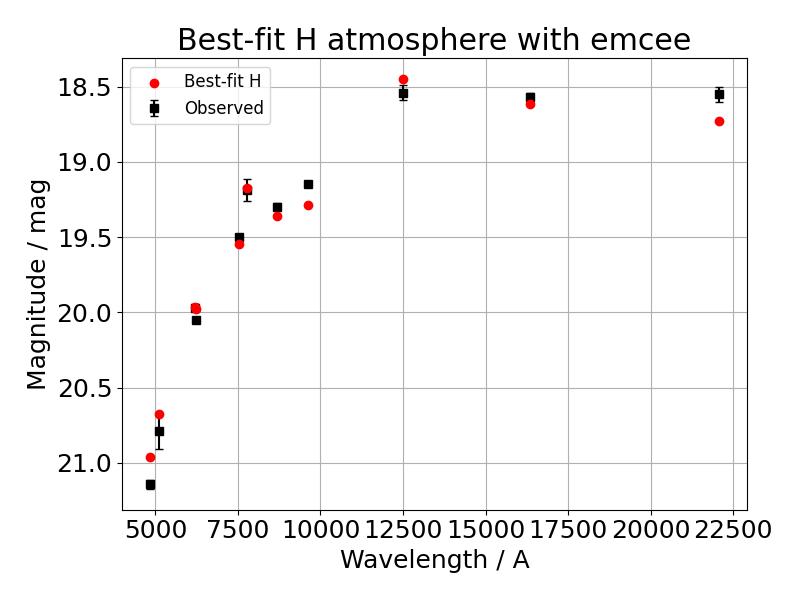
And the associated corner plot where the blue line shows the true value. As we are not providing a distance in this case, as expected from the degeneracy between fitting distance and stellar radius (directly translate to logg in the fit), both truth values are well outside of the probability density maps in the corner plot:

The options for the various models include:
- Kroupa 2001
- Charbrier 2003
- Charbrier 2003 (including binary)
- Manual
- PARSECz00001 - Z = 0.0001, Y = 0.249
- PARSECz00002 - Z = 0.0002, Y = 0.249
- PARSECz00005 - Z = 0.0005, Y = 0.249
- PARSECz0001 - Z = 0.001, Y = 0.25
- PARSECz0002 - Z = 0.002, Y = 0.252
- PARSECz0004 - Z = 0.004, Y = 0.256
- PARSECz0006 - Z = 0.006, Y = 0.259
- PARSECz0008 - Z = 0.008, Y = 0.263
- PARSECz001 - Z = 0.01, Y = 0.267
- PARSECz0014 - Z = 0.014, Y = 0.273
- PARSECz0017 - Z = 0.017, Y = 0.279
- PARSECz002 - Z = 0.02, Y = 0.284
- PARSECz003 - Z = 0.03, Y = 0.302
- PARSECz004 - Z = 0.04, Y = 0.321
- PARSECz006 - Z = 0.06, Y = 0.356
- GENEVAz002 - Z = 0.002
- GENEVAz006 - Z = 0.006
- GENEVAz014 - Z = 0.014
- MISTFem400 - [Fe/H] = -4.0
- MISTFem350 - [Fe/H] = -3.5
- MISTFem300 - [Fe/H] = -3.0
- MISTFem250 - [Fe/H] = -2.5
- MISTFem200 - [Fe/H] = -2.0
- MISTFem175 - [Fe/H] = -1.75
- MISTFem150 - [Fe/H] = -1.5
- MISTFem125 - [Fe/H] = -1.25
- MISTFem100 - [Fe/H] = -1.0
- MISTFem075 - [Fe/H] = -0.75
- MISTFem050 - [Fe/H] = -0.5
- MISTFem025 - [Fe/H] = -0.25
- MISTFe000 - [Fe/H] = 0.0
- MISTFe025 - [Fe/H] = 0.25
- MISTFe050 - [Fe/H] = 0.5
- Manual
- C08 - Catalan et al. 2008
- C08b - Catalan et al. 2008 (two-part)
- S09 - Salaris et al. 2009
- S09b - Salaris et al. 2009 (two-part)
- W09 - Williams, Bolte & Koester 2009
- K09 - Kalirai et al. 2009
- K09b - Kalirai et al. 2009 (two-part)
- C18 - Cummings et al. 2018
- EB18 - El-Badry et al. 2018
- Manual
L/I/H are used to denote the availability in the low, intermediate and high mass models, where the dividing points are at 0.5 and 1.0 solar masses.
The brackets denote the core type/atmosphere type/mass range/other special properties.
-
Montreal models
- Bedard et al. 2020 - LIH [CO/DA+DB/0.2-1.3]
-
LaPlata models
- Panei et al. 2007 - L [He+CO/DA/0.187-0.448]
- Althaus et al. 2009 - L [He/DA/0.220-0.521]
- Renedo et al. 2010 - I [CO/DA/0.505-0.934/Z=0.001-0.01]
- Althaus et al. 2015 - I [CO/DA/0.506-0.826/Z=0.0003-0.001]
- Althaus et al. 2017 - LI [CO/DA/0.434-0.838/Y=0.4]
- Camisassa et al. 2017 - I [CO/DB/0.51-1.0]
- Althaus et al. 2007 - H [ONe/DA/1.06-1.28]
- Camisassa et al. 2019 - H [ONe/DA+B/1.10-1.29]
-
BaSTI models
- Salaris et al. 2010 - IH [CO/DA+B/0.54-1.2/ps+nps]
-
MESA models
- Lauffer et al. 2018 - H [CONe/DA+B/1.012-1.308]
The following excerpt demonstrate how to generate luminosity functions with constant, burst and exponentially decaying
import os

from matplotlib import pyplot as plt
import numpy as np

from WDPhotTools import theoretical_lf

wdlf = theoretical_lf.WDLF()
wdlf.set_ifmr_model("C08")
wdlf.compute_cooling_age_interpolator()

mag = np.arange(0, 20.0, 0.1)
age_list = 1e9 * np.arange(2, 15, 2)

constant_density = []
burst_density = []
decay_density = []

for i, age in enumerate(age_list):

    # Constant SFR
    wdlf.set_sfr_model(mode="constant", age=age)
    constant_density.append(wdlf.compute_density(mag=mag)[1])

    # Burst SFR
    wdlf.set_sfr_model(mode="burst", age=age, duration=1e8)
    burst_density.append(wdlf.compute_density(mag=mag)[1])

    # Exponential decay SFR
    wdlf.set_sfr_model(mode="decay", age=age)
    decay_density.append(wdlf.compute_density(mag=mag)[1])

# normalise the WDLFs relative to the density at 10 mag
constant_density = [constant_density[i]/constant_density[i][Mag==10.0] for i in range(len(constant_density))]
burst_density = [burst_density[i]/burst_density[i][Mag==10.0] for i in range(len(burst_density))]
decay_density = [decay_density[i]/decay_density[i][Mag==10.0] for i in range(len(decay_density))]

fig1, (ax1, ax2, ax3) = plt.subplots(3, 1, sharex=True, sharey=True, figsize=(10, 15))

for i, age in enumerate(age_list):
    ax1.plot(
        mag, np.log10(constant_density[i]), label="{0:.2f} Gyr".format(age / 1e9)
    )
    ax2.plot(
        mag, np.log10(burst_density[i])
    )
    ax3.plot(
        mag, np.log10(decay_density[i])
    )

ax1.legend()
ax1.grid()
ax1.set_xlim(0, 20)
ax1.set_ylim(-3.75, 2.75)
ax1.set_title("Constant")

ax2.grid()
ax2.set_ylabel("log(arbitrary number density)")
ax2.set_title("100 Myr Burst")

ax3.grid()
ax3.set_xlabel(r"G$_{DR3}$ / mag")
ax3.set_title(r"Exponential Decay ($\tau=3\,Gyr$)")

plt.subplots_adjust(left=0.15, right=0.98, top=0.96, bottom=0.075)
plt.show()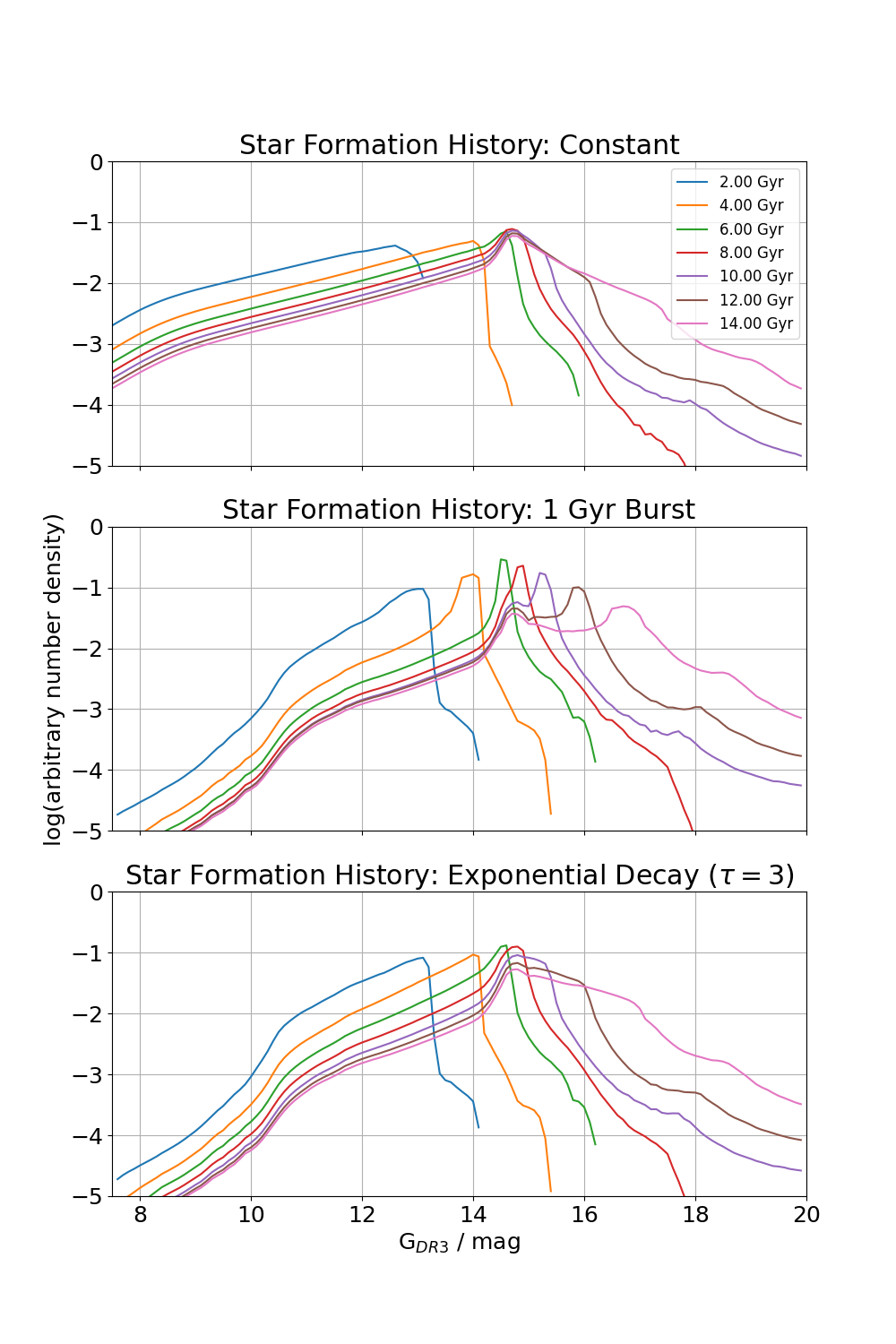

![dependabot-preview[bot] avatar](https://avatars.githubusercontent.com/in/2141?v=4 "dependabot-preview[bot]")


