eit-team/stroke_eit_dataset

Processing and directory structure for Stroke EIT Dataset

UCLH Stroke EIT Dataset

This Multifrequency Electrical Impedance Tomography (EIT) data was collected as part of clinical trial in collaboration with the Hyper Acute Stroke unit (HASU) at University College London Hospital (UCLH).

An overview of EIT along with a more detailed description of the data collection methodology and clinical context is given in the accompanying publication.

This repository contains the already processed data ready for analysis or use in imaging or classification studies, as well as the code to process all of the raw voltages.

Using Processed dataset

The processed data has been saved in JSON and MATLAB .mat formats. The steps to generate this data from the raw files is covered in the Processing Raw Data section.

MATLAB

Load the dataset using load('UCL_Stroke_EIT_Dataset.mat'). The data is stored in the structure EITDATA, with relevant settings saved in EITSETTINGS.

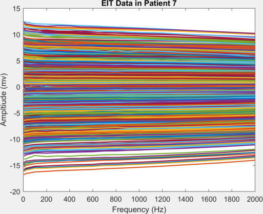
So for example, to plot the full spectrum data for patient 7

plot(EITSETTINGS.Freq,EITDATA(7).VoltagesCleaned)
xlabel('Frequency (Hz)');ylabel('Ampltiude (mv)');title('EIT Data in Patient 7');

Python (JSON data)

Loading data

import json

with open ("EITDATA.json") as json_file:
    EITDATA = json.load(json_file)

with open("EITSETTINGS.json") as json_file:
    EITSETTINGS = json.load(json_file)

Plotting data

Python array indexing starts at 0 (so array index 0 is patient 1). To plot the data from Patient 7 (as for MATLAB example), use index 6:

import matplotlib.pyplt as plt
plt.plot(EITDATA[6]['VoltagesCleaned']

Raw data files

The raw .bdf files are available should you wish to recreate or alter the processing of this dataset. In total the dataset is ~150GB, and is thus split into parts based on the Zenodo 50 GB file limit. Please download the following zip files and extract them into the corresponding folders.

• Subject data: into the ./Subjects folder
• Patient data (part 1): into the ./Patients folder
• Patient data (part 2): into the ./Patients folder
• Radiology data: into the ./Anonymised_Radiology folder

Example structures for these directories are given in the readmes.

Processing raw data

The data were collected using the UCL ScouseTom System archived at . All processing code is written in Matlab and is located in the Load_data repository archived at . Please ensure you follow the installation instructions there, and verify the example datasets load correctly. You may also find it easier to add ./src from this repository to the Matlab path.

The processing is done in two separate parts:

1. Demodulation - converting the "raw" sine waves into averaged impedance signals with magnitude and phase - uses the function ScouseTom_Load from Load_data.
2. Correction and extraction of real component - these are the form necessary for reconstruction. Extraction of the real part and normalisation for BioSemi gain and injected current amplitude is performed using normalised_dataset. Subsequently, rejection of poor quality measurements is performed using reject_channels. Both of these functions are found in this repository and an example is given in ./resource/Process_single_dataset.m.

Demodulation

For each subject and patient, there are three types of recordings:

1. Full spectrum "Multi-Frequency" datasets. These have the -MF suffix, e.g. S1a_MF1.bdf or P6-MF2.bdf. This used a 31 injection pair protocol with 17 frequencies and 3 frames.
2. Reduced spectrum "Time Difference" datasets. These have the -TD suffix e.g. S2b-TD1.bdf or P19-TD1.bdf. This has only 3 frequencies but was repeated for 60 frames.
3. Contact impedance checks or "Z Checks", with the suffix -Z e.g. S6-Z2.bdf or P11-Z4.bdf. Which injected current on neighbouring pairs of electrodes to estimate the contact impedance during electrode application.

The .bdf files contain the voltage data and the status of the digital trigger channels. Individual files can be demodulated like this:

ScouseTom_Load('./Subjects/Subject_01a/S1a_TD1.bdf')

or by calling ScouseTom_Load without any arguments and selecting a file.

1. Multi-Frequency datasets

These recordings used a 31 pair injection protocol, which was selected to maximise both the sensitivity inside the skull and the magnitude of the measured voltages (desc here). 17 frequencies were chosen to cover the range of the BioSemi and the expected contrast between healthy and stroke tissues. The full list is given below:

Freq (Hz)	Amp (uA)
5	45
10	45
20	45
100	45
200	90
300	90
400	90
500	90
600	90
700	140
800	140
900	140
1000	140
1200	160
1350	190
1700	235
2000	280

The current amplitude varied across frequency in accordance with IEC60601 and previous experience in low frequency measurements on the head.

To demodulate these recordings, call ScouseTom_Load('./Patients/Patient_11/P11_MF1.bdf') which saves a .mat file FNAME-BV.mat containing the demodulated voltages, as well as all other data relating to this dataset - EIT system setup, protocol, filtering parameters etc.

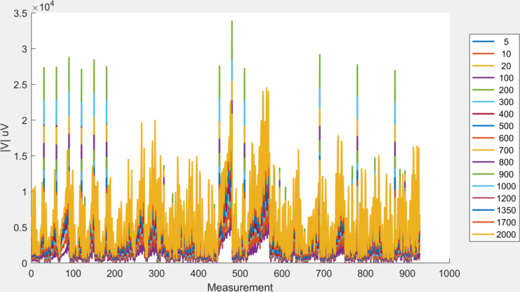
To load and plot this data:

figure
hold on
for iFreq = 1:size(ExpSetup.Freq,1)
    plot(mean(BV{iFreq}(keep_idx,:),2)) % keep_idx uses only channels
end
hold off
xlabel('Measurement');
ylabel('|V| uV')
legend(num2str(ExpSetup.Freq),'Location','eastoutside')

2. Time Difference datasets

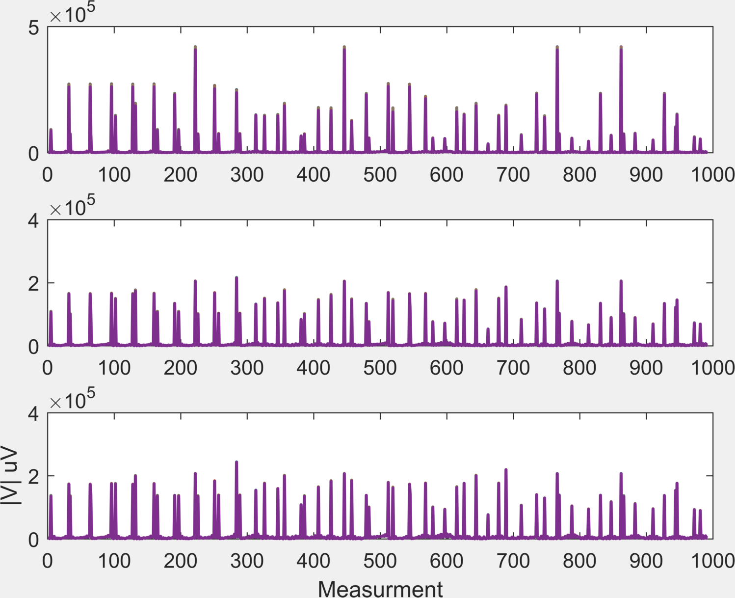
These recordings used the same injection protocol as the "Multi-Frequency" recordings, with only 3 frequencies: 200, 1200 2000 Hz. As with the MF dataset, use ScouseTom_Load('./Patients/Patient_17/P17_TD1.bdf'); to create file FNAME-BV.mat, which (for this example) can be loaded through the command: load('./Patients/Patient_17/P17_TD1-BV.mat'). You can plot these results like so: subplot(3,1,1);plot(BV{1});subplot(3,1,2);plot(BV{2});subplot(3,1,3);plot(BV{3});xlabel('Measurement');ylabel('|V| uV');

3. Contact Impedance Checks

To estimate the contact impedance at the electrode sites, a separate measurement protocol was used. This injected between all adjacent pairs of electrodes, in the same manner as the UCH Mk.2.5 system used in previous stroke studies .

Unlike the other data types, there is no accompanying log files, as every file uses the same protocol, injecting between consecutive neighbouring pairs 1-2,2-3,3-4...32-1 with a current of 1 kHz and 141 uA amplitude. The results of this are used as an indicator of the quality of the electrode contact. These were run repeatedly during electrode application until the contact was satisfactory. The final Z check (with the highest number) is run after all other data collection, to give an estimate of the drift in contact impedance during the recording.

These can be processed using the following:

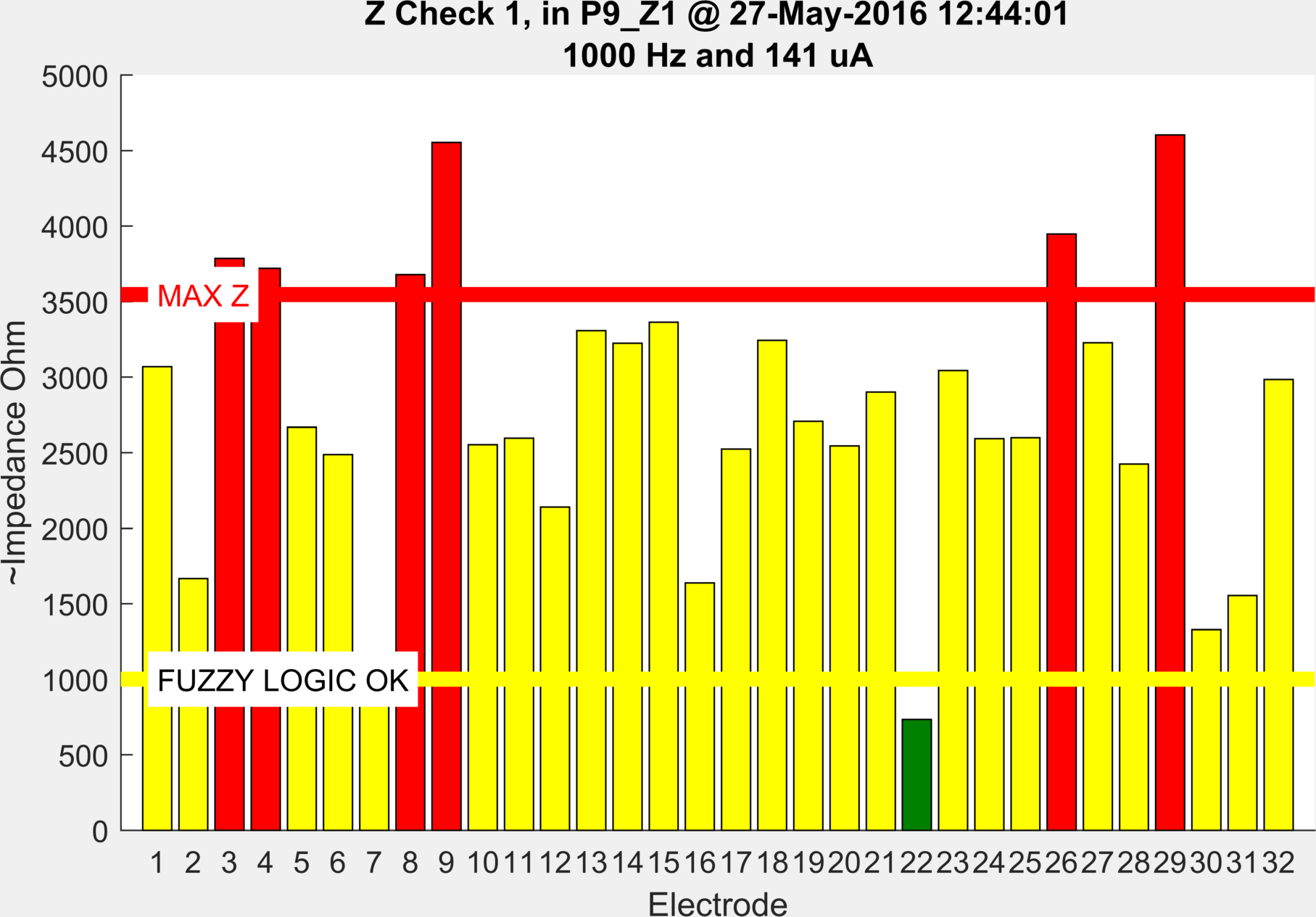
ScouseTom_Load('./Patients/Patient_09/P9_Z1.bdf') This shows an initial contact impedance check where electrodes 3,4,8,9,26,29 were too high. Prompting a reabrasion of the electrode site.

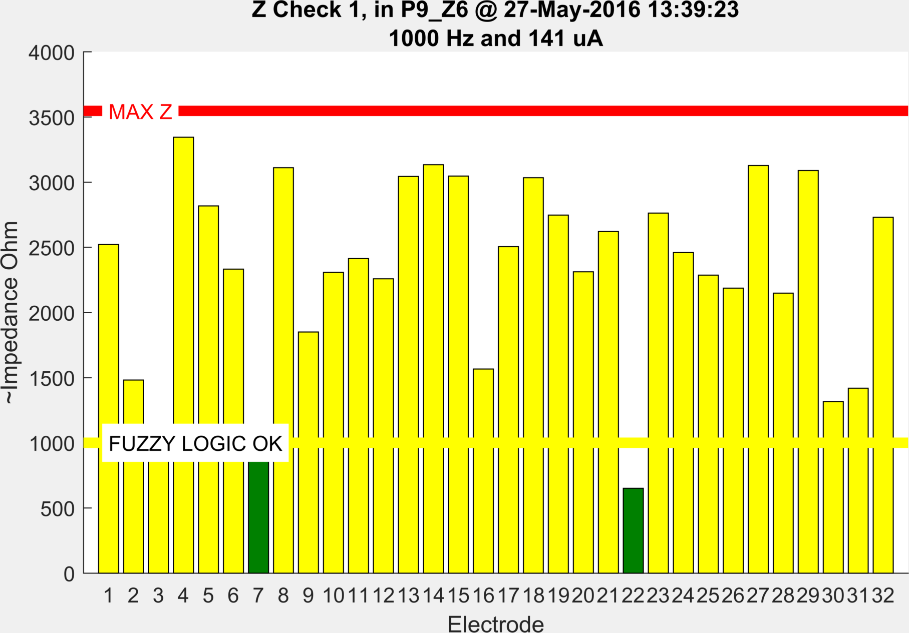
ScouseTom_Load('./Patients/Patient_09/P9_Z6.bdf') Shows the impedance at the end of the experiment where some have drifted over time, but none above the max Z level.

Correction and data rejection

Once all the data has been demodulated, and the FNAME-BV.mat file is produced (or using the ones already included). The voltages need to be corrected for the BioSemi gain and the changing injected current due to IEC 60601 (see system desc).

Assuming the /src directory is added to the Matlab path. The process is the same for either a MF or TD dataset, and takes two steps:

% correct for different gain across voltage
[BV, BVstruct]=normalise_dataset('./Patients/Patient_11/P11_MF1-BV.mat');
%pick a single frame - normally the 2nd is preferred for the full spectrum MF datasets.
[ BV_cleaned, chn_removed] = reject_channels( BV(:,:,2));

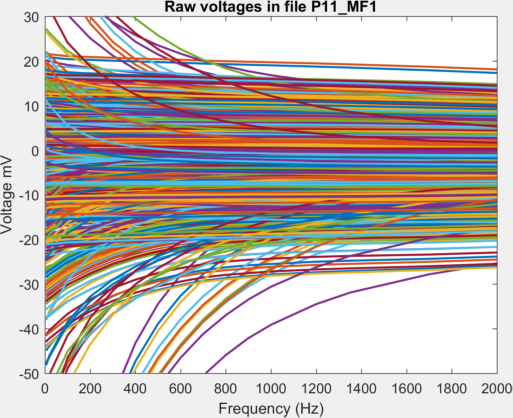
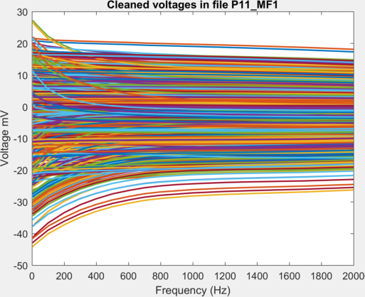
A complete example is given in Process_single_dataset.m. Which produces the following output:

• The raw voltages, showing some measurements with unusually high magnitude

• The cleaned voltages, with these channels removed

---

Batch Processing - Demodulation

All files for a given patient/subject can be processed using ScouseTom_ProcessBatch or ScouseTom_ProcessBatch('./Subjects/Subject_01a')

To demodulate all patients and all subjects, you can use the function ./resource/Demodulate_all.m which is located in this directory. Warning this takes a long time!

Batch Processing - Correction and data rejection

The final steps are given in ./resource/make_final_dataset.m, which corrects each dataset in turn and creates the final data structures EITDATA and EITSETTINGS stored in UCL_Stroke_EIT_Dataset.mat.

---

Example Mesh & Electrode coordinates

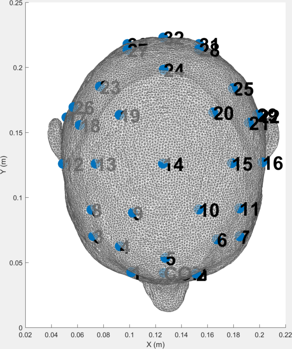
An example tetrahedral mesh is included in the resource folder, which is representative the of the type used in the UCL group in other studies. The electrode positions are given both as nominal X, Y, Z coordinates and in the EEG 10-10 system.

These can be visualised using the code ./resource/show_HASU_mesh.m

EEG Extraction

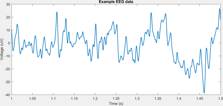
The portions of the dataset before and after EIT injection contain only EEG signals, which can be extracted through the use of Extract_EEG.m. This requires the raw data.

For example, to plot a segment of the EEG data at the beginning of the file

EEG=Extract_EEG('Subjects\Subject_06b\S6b_MF1.bdf');
plot(EEG.t_start,EEG.data_start(:,5)); xlim([1 1.5])
title('Example EEG data'); xlabel('Time (s)'); ylabel('Voltage (uV)')

Citing this work

Please use the corresponding publication to cite this data.

1. Goren, N. et al. Multi-frequency electrical impedance tomography and neuroimaging data in stroke patients. Sci. Data 5, 180112 (2018).

Please raise an issue or add to the wiki if you are interested in using this data. We would like to hear from you!

This work is licensed under a Creative Commons Attribution 4.0 International License.

stroke_eit_dataset's Issues

Tidy up Radiology folder

The .sh file can be removed and the instructions can be updated.

EITDATA file is corrupted

Please verify EITDATA.json file. It is corrupted and does not contain all data.

check positions of electrodes 26 and 29

The locations of electrodes 26 and 29 seems a bit off when ploted using show_HASU_mesh.m

DOI links missing

Example of using already processed data

Plotting example etc. in MATLAB/Python for .mat and .json files

Automatically add 'src' directory to MATLAB path

.

ScouseTom_TrigReadChn

I am currently trying to use the Extract_EEG function, but am getting a bad HDR error from the ScouseTom_TrigReadChn function on line 45.

`Error using ScouseTom_TrigReadChn (line 45)
Bad HDR

Error in Extract_EEG (line 33)
Trigger= ScouseTom_TrigReadChn(HDR);

Error in untitled2 (line 5)
EEG=Extract_EEG('Subjects\Subject_02b\S2b_MF1.bdf');`

Is there a work around for this?

Using Data in Python

Hi, I am currently trying to use this data for a project, and for my project I only really want the EEG data (i.e. the data extracted using Extract_EEG.m). Unfortunately, I do not know how to use this extracted data in Python for further use and processing. What is the best way to save this Extract_EEG data into BDF or CSV format just by itself (we want to use this with MNE)? Any input would be appreciated.

How do you recommend to EIT carrier frequency through low pass filtering

I am trying to extract EEG from the whole bdf using the low pass filtering that was recommended in the paper. How do you recommend we do this