A 3D electromagnetic FDTD simulator written in Python. The FDTD simulator has an optional PyTorch backend, enabling FDTD simulations on a GPU.
The fdtd-library can be installed with pip:
pip install fdtd
The development version can be installed by cloning the repository
git clone http://github.com/flaport/fdtd
and linking it with pip
pip install -e fdtd
Development dependencies can be installed with
pip install -e fdtd[dev]
- python 3.6+
- numpy
- scipy
- matplotlib
- tqdm
- pytorch (optional)
All improvements or additions (for example new objects, sources or detectors) are welcome. Please make a pull-request 😊.
read the documentation here: https://fdtd.readthedocs.org
The fdtd library is simply imported as follows:
import fdtdThe fdtd library allows to choose a backend. The "numpy" backend is the
default one, but there are also several additional PyTorch backends:
"numpy"(defaults to float64 arrays)"torch"(defaults to float64 tensors)"torch.float32""torch.float64""torch.cuda"(defaults to float64 tensors)"torch.cuda.float32""torch.cuda.float64"
For example, this is how to choose the "torch" backend:
fdtd.set_backend("torch")In general, the "numpy" backend is preferred for standard CPU calculations
with "float64" precision. In general, "float64" precision is always
preferred over "float32" for FDTD simulations, however, "float32" might
give a significant performance boost.
The "cuda" backends are only available for computers with a GPU.
The FDTD grid defines the simulation region.
# signature
fdtd.Grid(
    shape: Tuple[Number, Number, Number],
    grid_spacing: float = 155e-9,
    permittivity: float = 1.0,
    permeability: float = 1.0,
    courant_number: float = None,
)
A grid is defined by its shape, which is just a 3D tuple of Number-types
(integers or floats). If the shape is given in floats, it denotes the width,
height and length of the grid in meters. If the shape is given in integers, it
denotes the width, height and length of the grid in terms of the
grid_spacing. Internally, these numbers will be translated to three integers:
grid.Nx, grid.Ny and grid.Nz.
A grid_spacing can be given. For stability reasons, it is recommended to
choose a grid spacing that is at least 10 times smaller than the smallest
wavelength in the grid. This means that for a grid containing a source with
wavelength 1550nm and a material with refractive index of 3.1, the
recommended minimum grid_spacing turns out to be 50nm
For the permittivity and permeability floats or arrays with the following
shapes
(grid.Nx, grid.Ny, grid.Nz)- or
(grid.Nx, grid.Ny, grid.Nz, 1) - or
(grid.Nx, grid.Ny, grid.Nz, 3)
are expected. In the last case, the shape implies the possibility for different
permittivity for each of the major axes (so-called uniaxial or biaxial
materials). Internally, these variables will be converted (for performance
reasons) to their inverses grid.inverse_permittivity array and a
grid.inverse_permeability array of shape (grid.Nx, grid.Ny, grid.Nz, 3). It
is possible to change those arrays after making the grid.
Finally, the courant_number of the grid determines the relation between the
time_step of the simulation and the grid_spacing of the grid. If not given,
it is chosen to be the maximum number allowed by the Courant-Friedrichs-Lewy
Condition:
1 for 1D simulations, 1/√2 for 2D simulations and 1/√3 for 3D
simulations (the dimensionality will be derived by the shape of the grid). For
stability reasons, it is recommended not to change this value.
grid = fdtd.Grid(
    shape = (25e-6, 15e-6, 1), # 25um x 15um x 1 (grid_spacing) --> 2D FDTD
)
print(grid)
Grid(shape=(161,97,1), grid_spacing=1.55e-07, courant_number=0.70)
An other option to locally change the permittivity or permeability in the
grid is to add an Object to the grid.
# signature
fdtd.Object(
    permittivity: Tensorlike,
    name: str = None
)
An object defines a part of the grid with modified update equations, allowing
to introduce for example absorbing materials or biaxial materials for which
mixing between the axes are present through Pockels coefficients or many
more. In this case we'll make an object with a different permittivity than
the grid it is in.
Just like for the grid, the Object expects a permittivity to be a floats or
an array of the following possible shapes
(obj.Nx, obj.Ny, obj.Nz)- or
(obj.Nx, obj.Ny, obj.Nz, 1) - or
(obj.Nx, obj.Ny, obj.Nz, 3)
Note that the values obj.Nx, obj.Ny and obj.Nz are not given to the
object constructor. They are in stead derived from its placing in the grid:
grid[11:32, 30:84, 0] = fdtd.Object(permittivity=1.7**2, name="object")Several things happen here. First of all, the object is given the space
[11:32, 30:84, 0] in the grid. Because it is given this space, the object's
Nx, Ny and Nz are automatically set. Furthermore, by supplying a name to
the object, this name will become available in the grid:
print(grid.object) Object(name='object')
@ x=11:32, y=30:84, z=0:1
A second object can be added to the grid:
grid[13e-6:18e-6, 5e-6:8e-6, 0] = fdtd.Object(permittivity=1.5**2)Here, a slice with floating point numbers was chosen. These floats will be
replaced by integer Nx, Ny and Nz during the registration of the object.
Since the object did not receive a name, the object won't be available as an
attribute of the grid. However, it is still available via the grid.objects
list:
print(grid.objects)[Object(name='object'), Object(name=None)]
This list stores all objects (i.e. of type fdtd.Object) in the order that
they were added to the grid.
Similarly as to adding an object to the grid, an fdtd.LineSource can also be
added:
# signature
fdtd.LineSource(
period: Number = 15, # timesteps or seconds
amplitude: float = 1.0,
phase_shift: float = 0.0,
name: str = None,
)And also just like an fdtd.Object, an fdtd.LineSource size is defined by its
placement on the grid:
grid[7.5e-6:8.0e-6, 11.8e-6:13.0e-6, 0] = fdtd.LineSource(
period = 1550e-9 / (3e8), name="source"
)However, it is important to note that in this case a LineSource is added to
the grid, i.e. the source spans the diagonal of the cube defined by the slices.
Internally, these slices will be converted into lists to ensure this behavior:
print(grid.source) LineSource(period=14, amplitude=1.0, phase_shift=0.0, name='source')
@ x=[48, ... , 51], y=[76, ... , 83], z=[0, ... , 0]
Note that one could also have supplied lists to index the grid in the first
place. This feature could be useful to create a LineSource of arbitrary
shape.
# signature
fdtd.LineDetector(
name=None
)Adding a detector to the grid works the same as adding a source
grid[12e-6, :, 0] = fdtd.LineDetector(name="detector")print(grid.detector) LineDetector(name='detector')
@ x=[77, ... , 77], y=[0, ... , 96], z=[0, ... , 0]
# signature
fdtd.PML(
a: float = 1e-8, # stability factor
name: str = None
)Although, having an object, source and detector to simulate is in principle
enough to perform an FDTD simulation, One also needs to define a grid boundary
to prevent the fields to be reflected. One of those boundaries that can be
added to the grid is a Perfectly Matched
Layer or PML. These
are basically absorbing boundaries.
# x boundaries
grid[0:10, :, :] = fdtd.PML(name="pml_xlow")
grid[-10:, :, :] = fdtd.PML(name="pml_xhigh")
# y boundaries
grid[:, 0:10, :] = fdtd.PML(name="pml_ylow")
grid[:, -10:, :] = fdtd.PML(name="pml_yhigh")A simple summary of the grid can be shown by printing out the grid:
print(grid)Grid(shape=(161,97,1), grid_spacing=1.55e-07, courant_number=0.70)
sources:
LineSource(period=14, amplitude=1.0, phase_shift=0.0, name='source')
@ x=[48, ... , 51], y=[76, ... , 83], z=[0, ... , 0]
detectors:
LineDetector(name='detector')
@ x=[77, ... , 77], y=[0, ... , 96], z=[0, ... , 0]
boundaries:
PML(name='pml_xlow')
@ x=0:10, y=:, z=:
PML(name='pml_xhigh')
@ x=-10:, y=:, z=:
PML(name='pml_ylow')
@ x=:, y=0:10, z=:
PML(name='pml_yhigh')
@ x=:, y=-10:, z=:
objects:
    Object(name='object')
        @ x=11:32, y=30:84, z=0:1
Object(name=None)
@ x=84:116, y=32:52, z=0:1
Running a simulation is as simple as using the grid.run method.
grid.run(
    total_time: Number,
    progress_bar: bool = True
)
Just like for the lengths in the grid, the total_time of the simulation
can be specified as an integer (number of time_steps) or as a float (in
seconds).
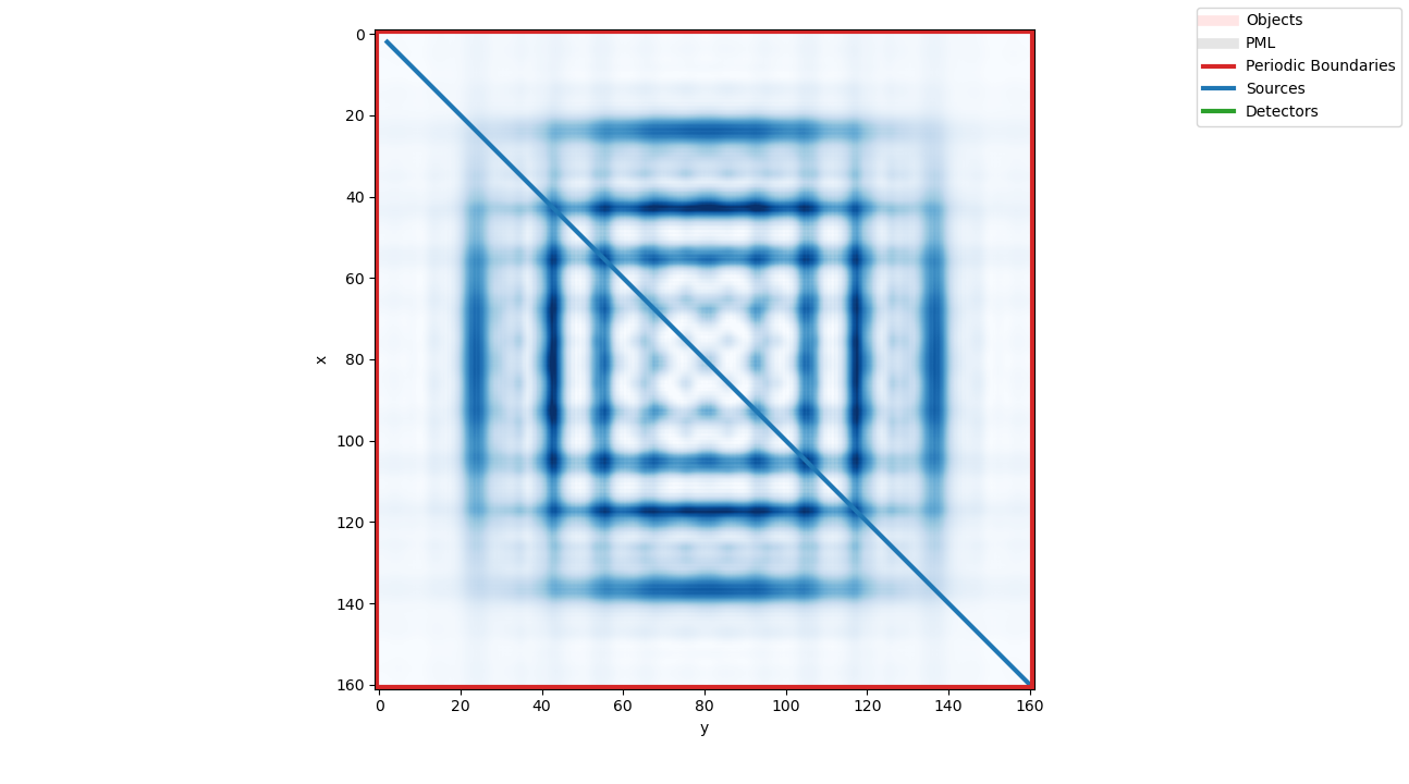
grid.run(total_time=100)Let's visualize the grid. This can be done with the grid.visualize method:
# signature
grid.visualize(
    grid,
    x=None,
    y=None,
    z=None,
    cmap="Blues",
    pbcolor="C3",
    pmlcolor=(0, 0, 0, 0.1),
    objcolor=(1, 0, 0, 0.1),
    srccolor="C0",
    detcolor="C2",
    show=True,
)
This method will by default visualize all objects in the grid, as well as the
field intensity at the current time_step at a certain x, y OR z-plane. By
setting show=False, one can disable the immediate visualization of the
matplotlib image.
grid.visualize(z=0)
An as quick as possible explanation of the FDTD discretization of the Maxwell equations.
An electromagnetic FDTD solver solves the time-dependent Maxwell Equations
    curl(H) = ε*ε0*dE/dt
    curl(E) = -µ*µ0*dH/dt
These two equations are called Ampere's Law and Faraday's Law respectively.
In these equations, ε and µ are the relative permittivity and permeability
tensors respectively. ε0 and µ0 are the vacuum permittivity and permeability
and their square root can be absorbed into E and H respectively, such that E := √ε0*E and H := √µ0*H.
Doing this, the Maxwell equations can be written as update equations:
    E  += c*dt*inv(ε)*curl(H)
    H  -= c*dt*inv(µ)*curl(E)
The electric and magnetic field can then be discretized on a grid with interlaced Yee-coordinates, which in 3D looks like this:

According to the Yee discretization algorithm, there are inherently two types
of fields on the grid: E-type fields on integer grid locations and H-type
fields on half-integer grid locations.
The beauty of these interlaced coordinates is that they enable a very natural way of writing the curl of the electric and magnetic fields: the curl of an H-type field will be an E-type field and vice versa.
This way, the curl of E can be written as
    curl(E)[m,n,p] = (dEz/dy - dEy/dz, dEx/dz - dEz/dx, dEy/dx - dEx/dy)[m,n,p]
                   =( ((Ez[m,n+1,p]-Ez[m,n,p])/dy - (Ey[m,n,p+1]-Ey[m,n,p])/dz),
                      ((Ex[m,n,p+1]-Ex[m,n,p])/dz - (Ez[m+1,n,p]-Ez[m,n,p])/dx),
                      ((Ey[m+1,n,p]-Ey[m,n,p])/dx - (Ex[m,n+1,p]-Ex[m,n,p])/dy) )
                   =(1/du)*( ((Ez[m,n+1,p]-Ez[m,n,p]) - (Ey[m,n,p+1]-Ey[m,n,p])), [assume dx=dy=dz=du]
                             ((Ex[m,n,p+1]-Ex[m,n,p]) - (Ez[m+1,n,p]-Ez[m,n,p])),
                             ((Ey[m+1,n,p]-Ey[m,n,p]) - (Ex[m,n+1,p]-Ex[m,n,p])) )
this can be written efficiently with array slices (note that the factor
(1/du) was left out):
def curl_E(E):
    curl_E = np.zeros(E.shape)
    curl_E[:,:-1,:,0] += E[:,1:,:,2] - E[:,:-1,:,2]
    curl_E[:,:,:-1,0] -= E[:,:,1:,1] - E[:,:,:-1,1]

    curl_E[:,:,:-1,1] += E[:,:,1:,0] - E[:,:,:-1,0]
    curl_E[:-1,:,:,1] -= E[1:,:,:,2] - E[:-1,:,:,2]

    curl_E[:-1,:,:,2] += E[1:,:,:,1] - E[:-1,:,:,1]
    curl_E[:,:-1,:,2] -= E[:,1:,:,0] - E[:,:-1,:,0]
    return curl_E
The curl for H can be obtained in a similar way (note again that the factor
(1/du) was left out):
def curl_H(H):
    curl_H = np.zeros(H.shape)

    curl_H[:,1:,:,0] += H[:,1:,:,2] - H[:,:-1,:,2]
    curl_H[:,:,1:,0] -= H[:,:,1:,1] - H[:,:,:-1,1]

    curl_H[:,:,1:,1] += H[:,:,1:,0] - H[:,:,:-1,0]
    curl_H[1:,:,:,1] -= H[1:,:,:,2] - H[:-1,:,:,2]

    curl_H[1:,:,:,2] += H[1:,:,:,1] - H[:-1,:,:,1]
    curl_H[:,1:,:,2] -= H[:,1:,:,0] - H[:,:-1,:,0]
    return curl_H
The update equations can now be rewritten as
    E  += (c*dt/du)*inv(ε)*curl_H
    H  -= (c*dt/du)*inv(µ)*curl_E
The number (c*dt/du) is a dimensionless parameter called the Courant number
sc. For stability reasons, the Courant number should always be smaller than
1/√D, with D the dimension of the simulation. This can be intuitively be
understood as the condition that information should always travel slower than
the speed of light through the grid. In the FDTD method described here,
information can only travel to the neighboring grid cells (through application
of the curl). It would therefore take D time steps to travel over the
diagonal of a D-dimensional cube (square in 2D, cube in 3D), the Courant
condition follows then automatically from the fact that the length of this
diagonal is 1/√D.
This yields the final update equations for the FDTD algorithm:
    E  += sc*inv(ε)*curl_H
    H  -= sc*inv(µ)*curl_E
This is also how it is implemented:
class Grid:
    # ... [initialization]

    def step(self):
        self.update_E()
        self.update_H()

    def update_E(self):
        self.E += self.courant_number * self.inverse_permittivity * curl_H(self.H)

    def update_H(self):
self.H -= self.courant_number * self.inverse_permeability * curl_E(self.E)Ampere's Law can be updated to incorporate a current density:
curl(H) = J + ε*ε0*dE/dtMaking again the usual substitutions sc := c*dt/du, E := √ε0*E and H := √µ0*H, the update equations can be modified to include the current density:
E += sc*inv(ε)*curl_H - dt*inv(ε)*J/√ε0Making one final substitution Es := -dt*inv(ε)*J/√ε0 allows us to write this
in a very clean way:
E += sc*inv(ε)*curl_H + EsWhere we defined Es as the electric field source term.
It is often useful to also define a magnetic field source term Hs, which would be
derived from the magnetic current density if it were to exist. In the same way,
Faraday's update equation can be rewritten as
H -= sc*inv(µ)*curl_E + Hsclass Source:
# ... [initialization]
def update_E(self):
# electric source function here
def update_H(self):
# magnetic source function here
class Grid:
# ... [initialization]
def update_E(self):
# ... [electric field update equation]
for source in self.sources:
source.update_E()
def update_H(self):
# ... [magnetic field update equation]
for source in self.sources:
source.update_H()When a material has a electric conductivity σ, a conduction-current will ensure that the medium is lossy. Ampere's law with a conduction current becomes
curl(H) = σ*E + ε*ε0*dE/dtMaking the usual substitutions, this becomes:
E(t+dt) - E(t) = sc*inv(ε)*curl_H(t+dt/2) - dt*inv(ε)*σ*E(t+dt/2)/ε0This update equation depends on the electric field on a half-integer time step (a
magnetic field time step). We need to substitute E(t+dt/2)=(E(t)+E(t+dt))/2 to
interpolate the electric field to the correct time step.
(1 + 0.5*dt*inv(ε)*σ/√ε0)*E(t+dt) = sc*inv(ε)*curl_H(t+dt/2) + (1 - 0.5*dt*inv(ε)*σ/ε0)*E(t)Which, yield the new update equations:
    f = 0.5*inv(ε)*σ*sc*du/(ε0*c)
    E *= inv(1 + f) * (1 - f)
    E += inv(1 + f)*sc*inv(ε)*curl_H
Note that the more complicated the permittivity tensor ε is, the more time consuming this algorithm will be. It is therefore sometimes a nice hack to transfer the absorption to the magnetic domain by introducing a (nonphysical) magnetic conductivity, because the permeability tensor µ is usually just equal to one:
    f = 0.5*inv(μ)*σm*sc*du/(μ0*c)
    H *= inv(1 + f) * (1 - f)
H += inv(1 + f)*sc*inv(µ)*curl_EThe electromagnetic energy density can be given by
e = (1/2)*ε*ε0*E**2 + (1/2)*µ*µ0*H**2making the above substitutions, this becomes in simulation units:
e = (1/2)*ε*E**2 + (1/2)*µ*H**2The Poynting vector is given by
P = E×HWhich in simulation units becomes
P = c*E×HThe energy introduced by a source Es can be derived from tracking the change
in energy density
de = ε*Es·E + (1/2)*ε*Es**2This could also be derived from Poyntings energy conservation law:
de/dt = -grad(S) - J·Ewhere the first term just describes the redistribution of energy in a volume and the second term describes the energy introduced by a current density.
Note: although it is unphysical, one could also have introduced a magnetic source. This source would have introduced the following energy:
de = ε*Hs·H + (1/2)*µ*Hs**2Since the µ-tensor is usually just equal to one, using a magnetic source term is often more efficient.
Similarly, one can also keep track of the absorbed energy due to an electric conductivity in the following way:
    f = 0.5*inv(ε)*σ*sc*du/(ε0*c)
    Enoabs = E + sc*inv(ε)*curl_H
    E *= inv(1 + f) * (1 - f)
    E += inv(1 + f)*sc*inv(ε)*curl_H
    dE = Enoabs - E
    e_abs += ε*E*dE + 0.5*ε*dE**2
or if we want to keep track of the absorbed energy by magnetic a magnetic conductivity:
    f = 0.5*inv(μ)*σm*sc*du/(μ0*c)
    Hnoabs = E + sc*inv(µ)*curl_E
    H *= inv(1 + f) * (1 - f)
    H += inv(1 + f)*sc*inv(µ)*curl_E
    dH = Hnoabs - H
    e_abs += µ*H*dH + 0.5*µ*dH**2
The electric term and magnetic term in the energy density are usually of the same size. Therefore, the same amount of energy will be absorbed by introducing a magnetic conductivity σm as by introducing a electric conductivity σ if:
inv(µ)*σm/µ0 = inv(ε)*σ/ε0Assuming we want periodic boundary conditions along the X-direction, then we
have to make sure that the fields at Xlow and Xhigh are the same. This has
to be enforced after performing the update equations:
Note that the electric field E is dependent on curl_H, which means that the
first indices of E will not be updated through the update equations. It's
those indices that need to be set through the periodic boundary condition.
Concretely: E[0] needs to be set to equal E[-1]. For the magnetic field,
the inverse is true: H is dependent on curl_E, which means that its last
indices will not be set. This has to be done by the boundary condition: H[-1]
needs to be set equal to H[0]:
class PeriodicBoundaryX:
    # ... [initialization]
    def update_E(self):
        self.grid.E[0, :, :, :] = self.grid.E[-1, :, :, :]

    def update_H(self):
        self.grid.H[-1, :, :, :] = self.grid.H[0, :, :, :]

class Grid:
    # ... [initialization]
    def update_E(self):
        # ... [electric field update equation]
        # ... [electric field source update equations]
        for boundary in self.boundaries:
            boundary.update_E()

    def update_H(self):
        # ... [magnetic field update equation]
        # ... [magnetic field source update equations]
        for boundary in self.boundaries:
boundary.update_H()a Perfectly Matched Layer (PML) is the state of the art for introducing absorbing boundary conditions in an FDTD grid. A PML is an impedance-matched absorbing area in the grid. It turns out that for a impedance-matching condition to hold, the PML can only be absorbing in a single direction. This is what makes a PML in fact a nonphysical material.
Consider Ampere's law for the Ez component, where we use the following substitutions:
E := √ε0*E, H := √µ0*H and σ := inv(ε)*σ/ε0 are
already introduced:
ε*dEz/dt + ε*σ*Ez = c*dHy/dx - c*dHx/dyThis becomes in the frequency domain:
iω*ε*Ez + ε*σ*Ez = c*dHy/dx - c*dHx/dyWe can split this equation in a x-propagating wave and a y-propagating wave:
    iω*ε*Ezx + ε*σx*Ezx = iω*ε*(1 + σx/iω)*Ezx = c*dHy/dx
    iω*ε*Ezy + ε*σy*Ezy = iω*ε*(1 + σy/iω)*Ezy = -c*dHx/dy
We can define the S-operators as follows
Su = 1 + σu/iω with u in {x, y, z}In general, we prefer to add a stability factor au and a scaling factor ku to Su:
Su = ku + σu/(iω+au) with u in {x, y, z}Summing the two equations for Ez back together after dividing by the respective S-operator gives
iω*ε*Ez = (c/Sx)*dHy/dx - (c/Sy)*dHx/dyConverting this back to the time domain gives
ε*dEz/dt = c*sx[*]dHy/dx - c*sx[*]dHx/dywhere sx denotes the inverse Fourier transform of (1/Sx) and [*] denotes a convolution.
The expression for su can be proven [after some derivation] to look as follows:
su = (1/ku)*δ(t) + Cu(t) with u in {x, y, z}where δ(t) denotes the Dirac delta function and C(t) an exponentially
decaying function given by:
Cu(t) = -(σu/ku**2)*exp(-(au+σu/ku)*t) for all t > 0 and u in {x, y, z}Plugging this in gives:
    dEz/dt = (c/kx)*inv(ε)*dHy/dx - (c/ky)*inv(ε)*dHx/dy + c*inv(ε)*Cx[*]dHy/dx - c*inv(ε)*Cx[*]dHx/dy
           = (c/kx)*inv(ε)*dHy/dx - (c/ky)*inv(ε)*dHx/dy + c*inv(ε)*Фez/du      with du=dx=dy=dz
This can be written as an update equation:
Ez += (1/kx)*sc*inv(ε)*dHy - (1/ky)*sc*inv(ε)*dHx + sc*inv(ε)*ФezWhere we defined Фeu as
Фeu = Ψeuv - Ψezw with u, v, w in {x, y, z}and Ψeuv as the convolution updating the component Eu by taking the derivative of Hw in the v direction:
Ψeuv = dv*Cv[*]dHw/dv with u, v, w in {x, y, z}This can be rewritten [after some derivation] as an update equation in itself:
     Ψeuv = bv*Ψeuv + cv*dv*(dHw/dv)
          = bv*Ψeuv + cv*dHw            with u, v, w in {x, y, z}
Where the constants bu and cu are derived to be:
    bu = exp(-(au + σu/ku)*dt)              with u in {x, y, z}
    cu = σu*(bu - 1)/(σu*ku + au*ku**2)     with u in {x, y, z}
The final PML algorithm for the electric field now becomes:
- Update
Фe=[Фex, Фey, Фez]by using the update equation for theΨ-components. - Update the electric fields the normal way
- Add
Фeto the electric fields.
or as python code:
class PML(Boundary):
    # ... [initialization]
    def update_phi_E(self): # update convolution
        self.psi_Ex *= self.bE
        self.psi_Ey *= self.bE
        self.psi_Ez *= self.bE

        c = self.cE
        Hx = self.grid.H[self.locx]
        Hy = self.grid.H[self.locy]
        Hz = self.grid.H[self.locz]

        self.psi_Ex[:, 1:, :, 1] += (Hz[:, 1:, :] - Hz[:, :-1, :]) * c[:, 1:, :, 1]
        self.psi_Ex[:, :, 1:, 2] += (Hy[:, :, 1:] - Hy[:, :, :-1]) * c[:, :, 1:, 2]

        self.psi_Ey[:, :, 1:, 2] += (Hx[:, :, 1:] - Hx[:, :, :-1]) * c[:, :, 1:, 2]
        self.psi_Ey[1:, :, :, 0] += (Hz[1:, :, :] - Hz[:-1, :, :]) * c[1:, :, :, 0]

        self.psi_Ez[1:, :, :, 0] += (Hy[1:, :, :] - Hy[:-1, :, :]) * c[1:, :, :, 0]
        self.psi_Ez[:, 1:, :, 1] += (Hx[:, 1:, :] - Hx[:, :-1, :]) * c[:, 1:, :, 1]

        self.phi_E[..., 0] = self.psi_Ex[..., 1] - self.psi_Ex[..., 2]
        self.phi_E[..., 1] = self.psi_Ey[..., 2] - self.psi_Ey[..., 0]
        self.phi_E[..., 2] = self.psi_Ez[..., 0] - self.psi_Ez[..., 1]

    def update_E(self): # update PML located at self.loc
        self.grid.E[self.loc] += (
            self.grid.courant_number
            * self.grid.inverse_permittivity[self.loc]
            * self.phi_E
        )

class Grid:
    # ... [initialization]
    def update_E(self):
        for boundary in self.boundaries:
            boundary.update_phi_E()
        # ... [electric field update equation]
        # ... [electric field source update equations]
        for boundary in self.boundaries:
            boundary.update_E()
The same has to be applied for the magnetic field.
These update equations for the PML were based on Schneider, Chap. 11.
As a bare FDTD library, this is dimensionally agnostic for any unit system you may choose. No conversion factors are applied within the library API; this is left to the user. (The code used to calculate the Courant limit may be a sticking point depending on the time scale involved).
However, as noted above (H := õ0*H), it is generally good numerical practice to scale all values to
get the maximum precision from floating-point types.
In particular, a scaling scheme detailed in "Novel architectures for brain-inspired photonic computers", Chapters 4.1.2 and 4.1.6, is highly recommended.
A set of conversion functions to and from reduced units are available for users in conversions.py.
You can run a linter in the root using pylint fdtd.
© Floris laporte - MIT License