Data Science Preparation

P.S. Ctrl+F to serach for relevant keywords.

Preliminaries

If you are just beginning with ML & Data Science, a good first place to start will be

Andrew Ng Coursera ML course. Finish at least the first few weeks.

If you have already done the Andrew Ng course, you might want to brush up on the concepts through these notes.

Notes on Andrew Ng Machine Learning

If you want to make a list of important interview topics head over to this article.

Machine Learning Cheatsheet

Courses & Resources

Data Science Practice Questions

If you are clueless about which topic to start from in data science, but have some basic idea about ML, then simply give these questions a go. If you get a bunch of them wrong, you'll know where to start your preparation :)

SQL

Quickly go through the tutorial pages, you need not cram anything. Soon after, solve all the Hackerrank questions (in sequence, without skipping). Refer back to any of the tutorials or look up the discussion forum when stuck. You will learn more effectively this way and applying the various clauses will boost your recall.

Probability

Statistics

Why divide by n-1 in sample standard deviation

Let f(v) = sum( (x_i-v)^2 )/n. Using f'(v) = 0, minima occurs at v = sum(x_i)/n = sample mean
Thus, f(sample mean) < f(population mean), as minima occurs at sample mean
Thus, sample std < population std (when using n in denominator)
But our goal was to estimate a value close to population std using the data of samples.
So we bump us sample std a bit by decreasing its denominator to n-1. Thus, bringing sample std closer to population std

Generative vs Discriminative models, Prior vs Posterior probability

Prior: Pr(x) assumed distirbution for the param to be estimated without accounting for obeserved (sample) data
Posterior: Pr(x | obsvd data) accounting for the observed data
Likelihood: Pr(obsvd data | x) P(x|obsvd data) ---proportional to--- P(obsvd data|x) * P(x) posterior ---proportional to--- likelihood * prior

Linear Algebra

Eigenvectors and eigenvalues | Essence of linear algebra, chapter 14

Distributions

(1) Exponential and Laplace Distributions
Gamma
Exponential
Students' T

Inferential Statistics

Notes on p-values, statistical significance

p-values
- 0 <= p-value <= 1
- The closer the p-value to 0, the more the confidence that the null hypothesis (that there is no difference between two things) is false.
- Threshold for making the decision: 0.05. This means that if there is no difference between the two things, then and the same experiment is repeated a bunch of times, then only 5% of them would yield a wrong decision.
- In essence, 5% of the experiments, where the differences come from weird random things, will generate a p-value less that 0.05.
- Thus, we should obtain large p-values if the two things being compared are identical.
- Getting a small p-value even when there is no difference is known as a False positive.'
- If it is extremely important when we say that the two things are different, we use a smaller threshold like 0.1%.
- A small p-value does not imply that the difference between the two things is large.
Error Types
- Type-1 error: Incorrectly reject null (False positive)
- Alpha: Prob(type-1 error) (aka level of significance)
- Type-2 error: Fail to reject when you should have rejected null hypothesis (False negative)
- Beta: Prob(type-2 error)
- Power: Prob(Finding difference between when when it truly exists) = 1 - beta
- Having power > 80% for a study is good. Calculated before study is conducted based on projections.
- P-value: Prob(obtaining a result as extreme as the current one, assuming null is true)
- Low p-value -> reject null hypothesis, high p-value -> fail to reject hypothesis
- If p-value < alpha -> study was statistically significant. Alpha = 0.05 usually

Maximum Likelihood Notes

Goal of maximum likelihood is to find the optimal way to fit a distribution to the data.
Probability: Pr(x | mu,std): area under a fixed distribution
Likelihood: Pr(mu,std | x) : y-axis values on curve (distribution function that can be varied) for fixed data point

Statistical Tests

t-Test

- compares 2 means. Works well when sample size is small. We esimate popl_std by sample_std.

- We are less confident that the distribution resembles normal dist. As sample size increases, it approches normal dist (at about n~=30)

- t-value = signal/noise = (absolute diff bet two means)/(variability of groups) = | x1 - x2 | / sqrt(s1^2/n1  +  s2^2/n2)

- Thus, increasing variance will give you more noise. Increasing #samples will decrease the noise.

- Degrees of freedom (DOF) = n1 + n2 - 2

- if t-value > critical value (from table) => reject hypothesis (found a statistically significant diff bet two means) 

- Independent (unpaired) samples means that two separate populations used to take samples. Paired samples means samples taken from the same population, and now we are comparing two means.

- In a two tailed test, we are not sure which direction the variance will be. Considering alpha=0.05, the 0.05 is split into 0.025 on both of the tails. In the middle is the remaining 0.95. Run a one-tailed test if sure about the directionality.

- (mu, sigma) are population statistics. (x_bar, s) are sample statistics.
- Calculating t-statistic when comparing sample mean with an already known mean. t-statistic = (x_bar - mu)/ sqrt(s^2/n)

Z-test

- Z-test uses a normal distribution

- (mu, sigma) are population statistics. (x_bar, s) are sample statistics. 

- z-score = (x-mu)/sigma  // no. of std dev a particular sample (x) is away from population mean
- z-statistic = (x_bar - mu)/ sqrt(sigma^2/n) // no. of std dev sample mean is away from population mean
- t-statistic = (x_bar - mu)/ sqrt(s^2/n) // when population std dev (sigma) is unavailable we substitute with sample std dev (s)

- Use z-stat when pop_std (sigma) is known and n>=30. Otherwise use t-stat.

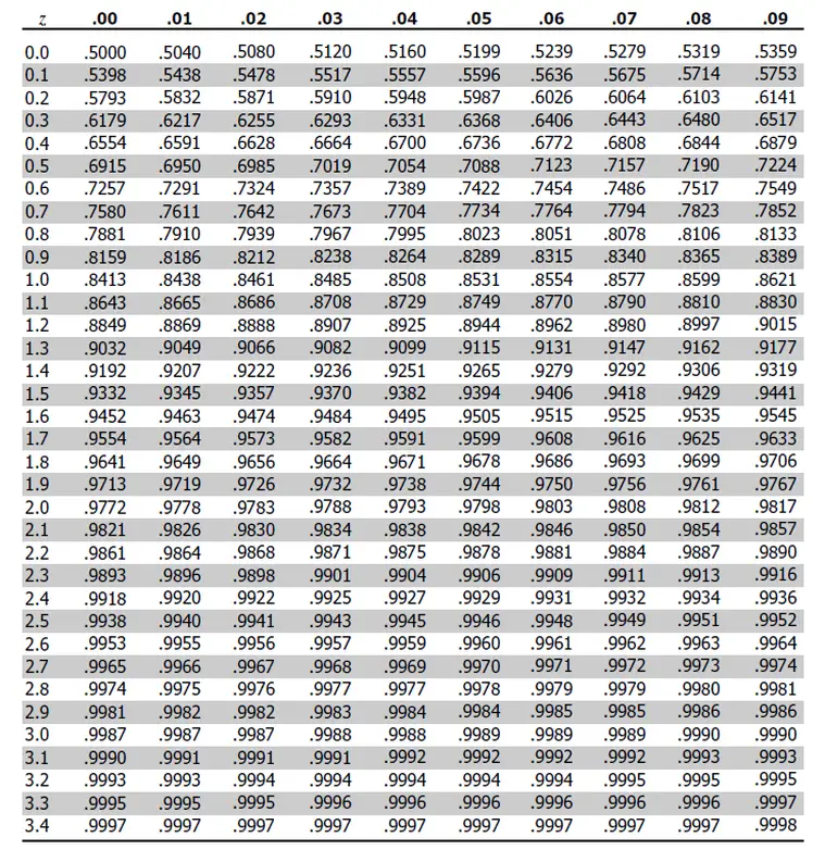
Z-test example

Z-score table
Question: Find z-critical score for two tailed test at alpha=0.03
- This means rejection area on each tail = 0.03/2 = 0.015
- So cumulative area till critical point on right = 1-0.015 = 0.985
- Now look for value on vertical axis that corresponds to 0.985 on alpha=0.03 column
- That value = 2.1 (z-critical score)

Chi-squred test

- chi^2 = sum( (observed-expected)^2 / (expected) )
- The larger the chi^2 value, the more likely the variables are related
- Correlation relationship between two attributes, A and B. A has c distinct values and B has r
- Contingency table: c values of A are the columns and r values of B the rows
- (Ai ,Bj): joint event that attribute A takes on value ai and attribute B takes on value bj
- oij= observed frequency, eij= expected frequency
- Test is based on a significance level, with (r -1)x(c-1) degrees of freedom
- Slides link: https://imgur.com/a/U4uJhHc

Statistical Tests notes

ANOVA test: compares >2 means
Chi-squared test: compares categorical variables
Shapiro Wilk test: test if a random sample comes from a normal distribution
Kolmogorov-Smirnov Goodness of Fit test: compares data with a known distribution to check if they have the same distribution

Linear Regression & Logistic Regression

Precision, Recall

Important Formulae

Sensitivity = True Positive Rate = TP/(TP+FN) = how sensitive is the model, same as recall
Specificity = 1 - False Positive Rate = 1 - FP/(FP+TN) = TN/(FP+TN)
'P'recision = TP/(TP+FP) = TP / 'P'redicted Positive = how less often does the model raise a false alarm
'R'ecall = TP/(TP+FN) = TP / 'R'eal Positive = of all the true cases, how many did we catch
F1-score = 2PrecisionRecall/(Precision + Recall) = geometric mean of precision & recall

ROC and AUC!
How to Use ROC Curves and Precision-Recall Curves for Classification in Python
F1 score, specificity, sensitivity

Gradient Descent

Stochastic Gradient Descent

Decision Trees & Random Forests

Information Gain

Information gain determines the reduction of the uncertainty after splitting the dataset on a particular feature such that if the value of information gain increases, that feature is most useful for classification.
IG = entropy before splitting - entropy after spliting
Entropy = - sum_over_n ( p_i * ln2(p_i) )

Gini Index

Higher the GI, more randomness. An attribute/feature with least gini index is preferred as root node while making a decision tree.
0: all elements correctly divided
1: all elements randomly distributed across various classes
0.5: all elements uniformly distributed into some classes
GI (P) = 1 - sum_over_n(p_i^2) where
P=(p1 , p2 ,.......pn ) , and pi is the probability of an object that is being classified to a particular class.

Loss functions

Cross entropy loss

 - Cross entropy loss for class X = -p(X) * log q(X), where p(X) = prob(class X in target), q(X) = prob(class X in prediction)
 - E.g. labels: [cat, dog, panda], target: [1,0,0], prediction: [0.9, 0.05, 0.05]
 - Total CE loss for multi-class classification is the summation of CE loss of all classes
 - Binary CE loss = -p(X) * log q(X) - (1-p(X)) * log (1-q(X))
 - Cross entropy loss works even for target like [0.5, 0.1, 0.4] as we are taking the sums of CE loss of all classes
 - In multi-label classification target can be [1, 0, 1] (not one-hot encoded). Given prediction: [0.6, 0.7, 0.4]. Then CE loss is evaluated as
   - CE loss A = Binary CE loss with p(X) = 1, q(X) = 0.6
   - CE loss B = Binary CE loss with p(X) = 0, q(X) = 0.7
   - CE loss B = Binary CE loss with p(X) = 1, q(X) = 0.4
   - Total CE loss = CE loss A + CE loss B + CE loss B

L1, L2 Regression

PCA, SVM, LDA

PCA

- Create a covariance matrix of the variables. Its eigenval and eigenvec describe the full multi-dimensional dataset.
- Eigenvec describe the direction of spread, Eigenval describe the importance of certain directions in describing the spread.
- In PCA, sequentially determine the axes in which the data varies the most
- All selected axes are eigenvectors of the symmetric covariance matrix, thus they are mutually perpendicular
- Then reframe the data using a subset of the most influential axes, by plotting the projections of original points on these axes. Thus dimensional reduction.
- Singular Value Decomposition is a way to find those vectors

SVM

- Margin is the smallest distance between decision boundary and data point.

- Maximum margin classifiers classify by using a decision boundary placed such that margin is maximized. Thus, they are super sensitive to outliers.

- Thus, when we allow some misclassifications to accomodate outliers, it is know as a Soft Margin Classifier aka Support Vector Classifier (SVC).

- Soft margin is determined through cross-validation. Support Vectors are those observations on the edge of Soft Margin.

- For 3D data, the Support Vector Classifier forms a plane. For 2D it forms a line.

- Support Vector Machines (SVM) moves the data into a higher dimension (new dimensions added by applying transformation on original dimensions)

- Then, a support vector classifier is found that separates the higher dimensional data into two groups.

- SVMs use Kernels that systematically find the SVCs in higher dimensions.

- Say 2D data transformed to 3D. Then Polynomial Kernels find 3D relationships between each pair of those 3D points. Then use them to find an SVC.

- Radial Basis Function (RBF) Kernel finds SVC in infinite dimensions. It behavs like a weighted nearest neighbour model (closest observations have the most impact on classification)

- Kernel functions do not need to transform points to higher dimenstion. They find pair-wise relationship between points as if they were in higher dimensions, known as Kernel Trick

- Polynomial relationship between two points a & b: (a*b + r)^d, where r & d are co-eff and degree of polynomial respectively found using cross validation

- RBF relationship between two points a & b: exp(-r (a-b)^2 ), where r determined using cross validation, scales the influence (in the weighted-nearest neighbour model)

Boosting

Adaboost

- Combines a lot of "weak learners" to make decisions.

- Single level decision trees (one root, two leaves), known as stumps.

- Each stump has a weighted say in voting (as opposed to random forests where each tree has an equal vote).

- Errors that the first stump makes, influences how the second stump is made. 
- Thus, order is important (as opposed to random forests where each tree is made independent of the others, doesnt matter the order in which trees are made)

- First all samples are given a weight (equal weights initially).
- Then first stump is made based on which feature classifies the best (feature with lowest Gini index chosen).
- Now to decide stump's weight in final classification, we calculate the following. 

- total_error = sum(weights of samples incorrectly classified)
- amount_of_say = 0.5log( (1-total_error)/total_error )

- When stump does a good job, amount_of_say is closer to 1.

- Now modify the weights so that the next stump learns from the mistakes.
- We want to emphasize on correctly classifying the samples that were wronged earlier.

- new_sample_weight = sample_weight * exp(amount_of_say) => increased sample weight
- new_sample_weight = sample_weight * exp(-amount_of_say) => decreased sample weight

- Then normalize new_sample_weights.
- Then create a new collection by sampling records, but with a greater probablilty of picking those which were wrongly classified earlier.
- This is where you can use new_sample_weights (normalized). After re-sampling is done, assign equal weights to all samples and repeat for finding second stump.

Gradient Boost

- Starts by making a single leaf instead of a stump. Considering regression, leaf contains average of target variable as initial prediction.
    
- Then build a tree (usu with 8 to 32 leaves). All trees are scaled equally (unlike AdaBoost where trees are weighted while prediciton)

- The successive trees are also based on previous errors like AdaBoost.

- Using initial prediction, calculate distance from actual target values, call them residuals, and store them.

- Now use the features to predict the residuals. 
- The average of the values that finally end up in the same leaf is used as the predicted regression value for that leaf
- (this is true when the underlying loss function to be minimized is the squared residual fn.)

- Then 
- new_prediction = initial_prediction + learning_rate*result_from_tree1
- new_residual = target_value - new_prediction

- new_residual will be smaller than old_residual, thus we are taking small steps towards learning to predict target_value accurately

- Train new tree on the new_residual, add the result_from_tree2*learning_rate to new_prediction to update it. Rinse and repeat.

Quantiles

Clustering

Neural Networks

CNN notes

for data with grid like topology (1D audio, 2D image)
reduces params in NN through
- sparse interactions
- parameter sharing
  - CNN creates spatial features.
  - Image passed through CNN gives rise to a volume. Section of this volume taken through the depth represents features of the same part of image
  - Each feature in the same depth layer is generated by the same filter that convolves the image (same kernel, shared parameters)
- equivariant representation
  - f(g(x)) = g(f(x))
Types of layers
- Convolution layer - image convolved using kernels. Kernel applied through a sliding window. Depth of kernel = 3 for RGB image, 1 for grey-scale
- Activation Layer -

Notes V.2

Problems with NN and why CNN?
- The amount of weights rapidly becomes unmanageable for large images. For a 224 x 224 pixel image with 3 color channels there are around 150,000 weights that must be trained
- MLP (multi layer perceptrons) react differently to an input (images) and its shifted version — they are not translation invariant
- Spatial information is lost when the image is flattened into an MLP. Nodes that are close together are important because they help to define the features of an image
- CNN’s leverage the fact that nearby pixels are more strongly related than distant ones. Influence of nearby pixels analyzed using filters.
Filters
- reduces the number of weights
- when the location of these features changes it does not throw the neural network off
The convolution layers: Extracts features from the input The fully connected (dense) layers: Uses data from convolution layer to generate output
Why do CNN work efficiently?
- Parameter sharing: a feature detector in the convolutional layer which is useful in one part of the image, might be useful in other ones
- Sparsity of connections: in each layer, each output value depends only on a small number of inputs

[But what is a neural network? | Chapter 1, Deep learning] (https://www.youtube.com/watch?v=aircAruvnKk)
Gradient descent, how neural networks learn | Chapter 2, Deep learning
What is backpropagation really doing? | Chapter 3, Deep learning
Train-test splitting, Stratification
Regularization, Dropout, Early Stopping
Convolution Neural Networks - EXPLAINED
k-fold Cross-Validation
Exploding and vanishing gradients
Intro to CNN

gsunit / data-science-preparation Goto Github PK