jamesjscully/reservoircomputing.jl

Reservoir computing utilities for scientific machine learning (SciML)

ReservoirComputing.jl

Reservoir computing utilities

Installation

Usual Julia package installation. Run on the Julia terminal:

julia> using Pkg
julia> Pkg.add("ReservoirComputing")

Echo State Network example

This example and others are contained in the examples folder, which will be updated whenever I find new examples. To show how to use some of the functions contained in ReservoirComputing.jl, we will illustrate it by means of an example also shown in the literature: reproducing the Lorenz attractor. First, we have to define the Lorenz system and the parameters we are going to use:

using ParameterizedFunctions
using OrdinaryDiffEq
using ReservoirComputing

#lorenz system parameters
u0 = [1.0,0.0,0.0]                       
tspan = (0.0,200.0)                      
p = [10.0,28.0,8/3]
#define lorenz system
function lorenz(du,u,p,t)
    du[1] = p[1]*(u[2]-u[1])
    du[2] = u[1]*(p[2]-u[3]) - u[2]
    du[3] = u[1]*u[2] - p[3]*u[3]
end
#solve and take data
prob = ODEProblem(lorenz, u0, tspan, p)  
sol = solve(prob, ABM54(), dt=0.02)   
v = sol.u
data = Matrix(hcat(v...))
shift = 300
train_len = 5000
predict_len = 1250
train = data[:, shift:shift+train_len-1]
test = data[:, shift+train_len:shift+train_len+predict_len-1]

Now that we have the datam we can initialize the parameters for the echo state network:

approx_res_size = 300
radius = 1.2
degree = 6
activation = tanh
sigma = 0.1
beta = 0.0
alpha = 1.0
nla_type = NLAT2()
extended_states = false

Now it's time to initiate the echo state network:

esn = ESN(approx_res_size,
    train,
    degree,
    radius,
    activation = activation, #default = tanh
    alpha = alpha, #default = 1.0
    sigma = sigma, #default = 0.1
    nla_type = nla_type, #default = NLADefault()
    extended_states = extended_states #default = false
    )

The echo state network can now be trained and tested:

W_out = ESNtrain(esn, beta)
output = ESNpredict(esn, predict_len, W_out)

ouput is the matrix with the predicted trajectories that can be easily plotted

using Plots
plot(transpose(output),layout=(3,1), label="predicted")
plot!(transpose(test),layout=(3,1), label="actual")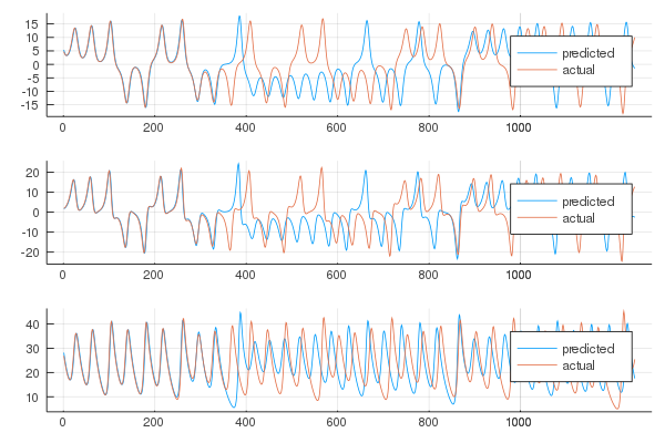

One can also visualize the phase space of the attractor and the comparison with the actual one:

plot(transpose(output)[:,1], transpose(output)[:,2], transpose(output)[:,3], label="predicted")
plot!(transpose(test)[:,1], transpose(test)[:,2], transpose(test)[:,3], label="actual")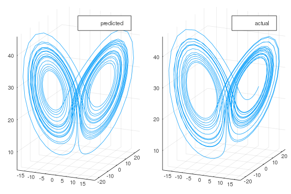

The results are in line with the literature.

The code is partly based on the original paper by Jaeger, with a few construction changes found in the literature. The reservoir implementation is based on the code used in the following paper, as well as the non-linear transformation algorithms T1, T2, and T3, the first of which was introduced here.

To do list

• Documentation
• Implement variable number of outputs as in this paper
• Implement different systems for the reservoir (like this paper)