The aibecs.jl from juliaocean

Fix coverage

Probably mostly a cleaning-up task.

Issues with replicating documentation example

I was going through the AIBECS model with the example provided by the documentation. In the Radiocarbon dating example, I noticed that plotting function was not working as expected: It throws an error whenever I wanted to plot the horizontal slice graph:

plothorizontalslice(age_in_yrs, grd, depth=2000u"m", color=:magma)
ERROR: MethodError: no method matching plot(::AIBECS.HorizontalPlane; color=:magma)

Similar error is encountered in the horizontal mean plot. Do you know what when wrong there?

Thanks

Throw error when CTKAlg does not converge

This would allow me to spot the failing runs quicker.

Bugs in the doc examples must be corrected!

fix docs ideal age

"thgus" and age restoring in LaTeX is incorrect.

Precompute mismatch scaling factor

Specifically, refactor these to allow the user to provide transpose(o) * W * o instead of recalculating it every time:

AIBECS.jl/src/multiTracer.jl

Lines 321 to 355 in 960ecad

    
           ## new functions for more generic obs packages 
        
           # TODO Add an optional function argument to transform the data before computingn the mismatch 
        
           # Example if for isotope tracers X where one ususally wants to minimize the mismatch in δ or ε. 
        
           function mismatch(x, grd::OceanGrid, obs; c=identity, W=I, M=interpolationmatrix(grd, obs.metadata), iwet=iswet(grd, obs)) 
        
               o = view(obs, iwet) 
        
               δx = M * c(x) - o 
        
               return 0.5 * transpose(δx) * W * δx / (transpose(o) * W * o) 
        
           end 
        
           mismatch(x, grd::OceanGrid, ::Missing; kwargs...) = 0 
        
           function ∇mismatch(x, grd::OceanGrid, obs; c=identity, W=I, M=interpolationmatrix(grd, obs.metadata), iwet=iswet(grd, obs)) 
        
               ∇c = Diagonal(ForwardDiff.derivative(λ -> c(x .+ λ), 0.0)) 
        
               o = view(obs, iwet) 
        
               δx = M * c(x) - o 
        
               return transpose(W * δx) * M * ∇c / (transpose(o) * W * o) 
        
           end 
        
           ∇mismatch(x, grd::OceanGrid, ::Missing; kwargs...) = transpose(zeros(length(x))) 
        
           # In case the mismatch is not based on the tracer but on some function of it 
        
           function indirectmismatch(xs::Tuple, grd::OceanGrid, modify::Function, obs, i, M=interpolationmatrix(grd, obs[i].metadata), iwet=iswet(grd, obs[i])) 
        
               x2 = modify(xs...) 
        
               out = 0.0 
        
               M = interpolationmatrix(grd, obs[i].metadata) 
        
               iwet = iswet(grd, obs[i]) 
        
               o = view(obs[i], iwet) 
        
               δx = M * x2[i] - o 
        
               return 0.5 * transpose(δx) * δx / (transpose(o) * o) 
        
           end 
        
           function ∇indirectmismatch(xs::Tuple, grd::OceanGrid, modify::Function, obs, i, M=interpolationmatrix(grd, obs[i].metadata), iwet=iswet(grd, obs[i])) 
        
               nt, nb = length(xs), length(iswet(grd)) 
        
               x2 = modify(xs...) 
        
               o = view(obs[i], iwet) 
        
               δx = M * x2[i] - o 
        
               ∇modᵢ = ∇modify(modify, xs, i) 
        
               return transpose(δx) * M * ∇modᵢ / (transpose(o) * o) 
        
           end

Raise a warning instead of an error for reusing same parameters name

That would allow for a less painful devlopment experience.

Add tests to diagnostics

Fix docs plots with new recipes' aspect ratio defaullt

Some of the plots in the docs that have two maps concatenated in the same plot object have disproportionately large subplot frames/bboxes. Probably just setting size in the last plot call fixes it.

Move from using JLD2 to using BSON

JLD2 not being actively maintained is an issue. BSON.jl has been suggested a couple times already as being offering similar functionality, but is actively maintained, so I should use that instead.

Make sure F1Method paper runs work with AIBECS

TagBot trigger issue

This issue is used to trigger TagBot; feel free to unsubscribe.

If you haven't already, you should update your TagBot.yml to include issue comment triggers.
Please see this post on Discourse for instructions and more details.

Add Makie recipes

Leveraging MakieLayout, Makie seems posed to become the default plotting package for publication quality figures, so it would be great to add some Makie plot recipes, add tests, and some tutorials/how-to's that showcase these recipes.

Use JLD2 with compression instead of BSON for storage

Saving the OCIM2 grd and T using JLD2 with the {compress=true} flag reduces the file size from about 75 to 28 MB.

Merge into DifferentialEquations, NLSolve

I think in the long run it will be good to somehow merge the solving functionality of this package (the solver(s) in particular) with the well maintained packages of DifferentialEquations and/or NLSolve. This would provide lots of added functionality (e.g., for #4, #5, etc.). Also this might help to provide a DSL as suggested in #18

simplify single tracer usage

Add function to unpack state to 3D array(s)

Right now I do this via

const iDIP = 1:nb
const iDOP = iDIP .+ nb
const iPOP = iDOP .+ nb
function unpack_state(x)
DIP = x[iDIP]
DOP = x[iDOP]
POP = x[iPOP]
return DIP, DOP, POP
end

and

DIP, DOP, POP = unpack_state(x)

and

DIP_3d = NaN * wet3d; DIP_3d[iwet] = DIP

Probably good to have a unpack_state and vector_to_3D functions in AIBECS

Add generic diagnostics capability

Let's try to add some diagnostic functionality to AIBECS that generalizes the work done in Pasquier and Holzer, 2018.

Preliminary notes

Let's start from the generic equation

(∂ₜ + T) x = G(x).

x could represent a multitude of tracers and processes. Within x, there may be separate groups of tracers with a group per compound or element. E.g., one could be tracking many elements including, e.g., phosphorus, whose group could be composed of three pools, like PO₄, DOP, and POP. For the diagnostics that I am interested in, we will assume for simplicity and without any loss of generality, that there is only one element (one group) here.

We can then express the group's system without loss of generality as a bunch of

source terms s_p(x) that inject x into the system,
of "transfers" terms that exchange the element between tracers of our group J_i→j(x),
and of "death" processes d_q(x), which ultimately remove x from the system.

Mathematically, that means we can write

G(x) = ∑_p s_p(x) + ∑_ij J_i→j(x) + ∑_q d_q(x).

We construct the LEM by first creating linear-equivalent terms for J_i→j(x) and d_q(x), evaluated at the steady-state solution x given by

T x = G(x)

In other words, the LEM is built such that

G(x) = ∑_p s_p + ∑_ij L_i→j x + ∑_q L_q x

when x is the steady-state, and where

L_i→j is a block matrix where only 2 blocks are non-zero, (i,j) and (j,i), which have diagonals -(J_i→j(x))_i / x_i, and +(J_i→j(x))_j / x_i, respectively. (Note we use x_i to "linearize" J_i→j so that the rate of transfer is specific to the removed tracer.)
and L_q is a diagonal matrix with diagonal d_q(x) / x.

We then construct the LEM simply as

(∂ₜ + H) x = ∑_p s_p

where

H = T - ∑_ij L_i→j - ∑_q L_q

and we can then exploit this for powerful diagnostics as in Pasquier and Holzer, 2018. Fractions that came from source s_p, or fraction that will be removed via process d_q, are available from a single backslash with H. One can also further partition according to each i→j passage by removing J_i→j from H into a F operator and iteratively reapplying the source term. Direct computations leveraging the classical identities ∑_n xⁿ and ∑_n n xⁿ also allow for direct computations of, e.g., the number of i→j passages.

Allow for redefinition of Parameters

Maybe I can create a new name at each call of initialize_Parameters? E.g., Parameters_1, Parameters_2, etc.

logo ideas

AIBECS_logo_Cartopy.pdf

Revise ReadMe to match current state of the package

docs: Concept: Explicit local G and nonlocal T

I.e., the partition of the tracer equation into local sources and sinks and transport.

Plotting features

Add grant info from USC

Add ICBM circulation?

Plot Recipes refactor

Probably a good idea to bundle them into a submodule to control what's exported.

Also better to bring the factor out the computation part into OceanGrids. That is, have a zonalaverage function in OceanGrids, or maybe even an overload of StatsBase/Statistics' likemean(::ZonalAverage, x, grd) or sum(::ZonalIntegral, x, grd) to just spit out the array, and then have the recipes use those functions directly instead.

Add documentation

Memoize some functions

It might be beneficial performance-wise to memoize some functions with a single memory cache when running optimizations, especially if I can keep a lot in memory :) Memoize.jl seems to be able to do just that... From its ReadMe:

using Memoize
using LRUCache
@memoize LRU{Tuple{Any,Any},Any}(maxsize=2) function x(a, b)
    println("Running")
    a + b
end

Evaluate parameter cost in λ space

This might allow me to use LogitNormal as a prior.

Assume p has a D(p) = a + (b-a) * LogitNormal() prior. λ = subfun⁻¹(p) = logit((p - a) / (b - a)) (or is it the reverse) is then Normal() distributed in the sense that obj(λ) contains a -gradlogpdf(Normal(), λ) penalty. This is a priori great for Optim because this function is log-convex, real-valued — it's a quadratic afterall. However, when obj(λ) and its derivatives are computed, and subsequently λ is updated by Optim, if λ has been pushed a bit too far to one side, it may very well be that p = subfun(λ) is floating-arithmetic-rounded to be exactly a (or b), i.e., one of the bounds of the support of the prior. Then mismatch(p) = -gradlogpdf(D(p), a) evaluates to +Inf and everything falls apart. In reality, however, I don't think the mismatch should be that big, since it should just be -gradlogpdf(D(p), λ), and the penalty should ensure that this is not even close to +Inf. The solution could be to always evaluate the mismatch in λ space.

Side note/issue: Toying with TransformVariables, Bijectors, and what AIBECS does (in a local Pluto notebook that I should probably save as a gist and reference here), I noticed that I don't recover exactly what I'm supposed to going from p-space to λ-space in terms of gradlogpdf, so it would be good to elucidate that first before diving into this potential rabbit hole.

Add 2x2x2 Box model

Here is the schematic made by @louisprimeau

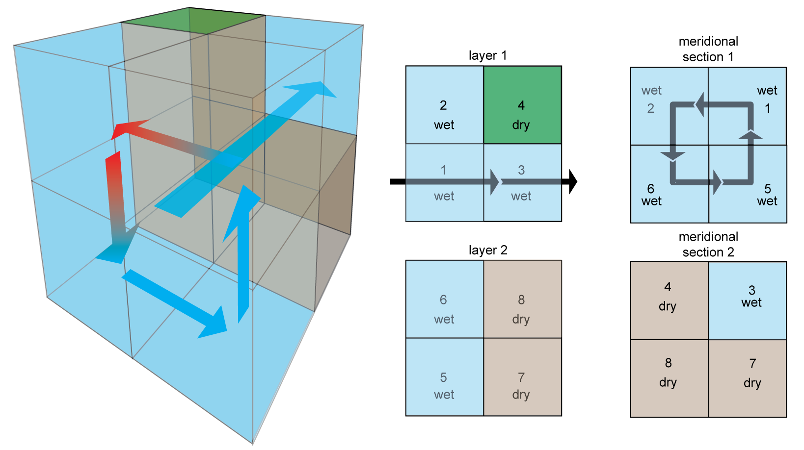
saved here for to be added to the corresponding notebook. (@fprimeau or @louisprimeau let me know if you want me to take it away from here.)

Time-steppers

Multigrid / coarse graining

It would be great to be able to coarse-grain any given matrix to allow for quick testing.

Not sure how to do this easily. In particular, making this generic might not be possible, in particular, if the fine grid has a non-easily divisible size in one dimension (e.g., OCIM2 has size 91 in latitude, which is divisible by 7 🤷), or if the coarse grid would bundle separate boxes together (e.g., boxes originally separated by land diagonally).

Krylov methods

Consider using ModelParameters.jl for parameters

See rafaqz/ModelParameters.jl#8 (comment) for reference.

Maybe try by building a small example AIBECS model manually and go from there.

Update OCIM2 files

Current OCIM2 files were built with UnitfulAstro's yr. While I don't think this is a problem for T and grd, it is one for the He fluxes, which are in mol/m^3/yr.

Todo list:

include mask into grid

It would make for a cleanar API to just do

julia> grid, T = OCIM1.load()

and have the wet point indices or the mask wet3D inside of grid.

This would mean breaking changes for

OceanGrid
AIBECS (tests and notebooks)
the BSON files on FigShare
the hash checksums on AIBECS for those files.

Rivers numerical noise

In the river tutorial, if I change the first solution plot to

cmap = :RdYlBu_4
plothorizontalslice(s, grd, zunit=u"μmol/m^3", depth=0, color=cmap, clim=(-1,1))

I get to see numerical noise at the Amazon outlet and other major rivers at the surface.

With OCIM2:

OCIM1:

OCCA:

Add 10/11-box PANDORA model

See doi: 10.1029/GB001i001p00015

Add a two-box model of the circulation

I find I could sometimes use a very simple 2-box model, so let's make one. Should probably go with the values in the Sarmiento and Gruber book or the reference therein, if any.

Add Kok et al dataset

Allow for long names of parameters to print nicely

Probably add something like

print_type(io, f, val::Float64, ppu, s, n) = @printf io "%$(n)s = %8.2e [%s] %s\n" f val ppu s

where n is the maximum length of all the symbols?

DSL with macros?

Maybe worth reworking the interface to be simpler and yielding more efficient code.
I was thinking of something along the lines of

Define tracers, e.g., DIP, DOP, POP, DFe, DO₂, maybe with a macro like
```
@define_tracers DIP DOP POP DFe DO₂
```

Then define functions and who they apply to, maybe something like

@add_BGC_sink DIP → uptake : 1 / τ * DIP^2 / (DIP + k) * (z ≤ zₑ)
@add_BGC_source POP : σ * uptake
@add_BGC_source DOP : (1-σ) * uptake
@add_BGC_transfer DOP → DIP : kDOP * DOP
@add_BGC_transfer POP → DOP : kPOP * POP
@add_restoring DIP : DIPgeo τgeo
@add_external_source DFe : aeolian_DFe_source
etc.

Then be able to pack/unpack the tracers and also create efficient inplace F (as suggested in #10)

Think about a generic grid type...

Maybe try to figure out what CLIMA peeps are doing and use that? Otherwise AxisArrays?

AIBECS `F` is quite slower (5x) than handmade `F`

Improve river tutorial

This tutorial needs a few improvements

Add a plot of the original-data sources and the mouth-location nearest-neghbor interpolation.
Chose a better colormap
find better things to plot
Make sure the output of code cells is not too long

AO functionality

A worthy successor to the AWESOME OCIM (AO) should include all the functionality of the AO.
I try to reuse the AO nomenclature for reference, and will update with AIBECS names if I change them.

Thi issue will serve me as a check/TODO list to incorporate things one can do in the AO into AIBECS:

use depth of bottom of boxes for sinking particles

I might want to change all the examples to use the depth at the bottom of the box to define w(p) instead of depthvec(grd).

Add feature to figure out independent tracers and use it

Assuming one wants to simulate two independent tracers at the same time, there is no need to construct the full matrix. A better approach is to split the model into separate sub-models. Maybe a good solution is to raise a warning if some tracers are independent. The user can then think of it as separate models with separate inputs and outputs, that can be combined after the fact if needed.

Add OCCA matrix

Fix transportoperator for OCCA matrix

I'm unsure at this stage but it seems to me that I should revisit the transport operator function to accommodate for the OCCA matrix because its cell volumes already account for subgrid topography (and the transport too?) and I think this causes mass-conservation problems for DIP–POP-like systems.

	## new functions for more generic obs packages
	# TODO Add an optional function argument to transform the data before computingn the mismatch
	# Example if for isotope tracers X where one ususally wants to minimize the mismatch in δ or ε.
	function mismatch(x, grd::OceanGrid, obs; c=identity, W=I, M=interpolationmatrix(grd, obs.metadata), iwet=iswet(grd, obs))
	o = view(obs, iwet)
	δx = M * c(x) - o
	return 0.5 * transpose(δx) * W * δx / (transpose(o) * W * o)
	end
	mismatch(x, grd::OceanGrid, ::Missing; kwargs...) = 0
	function ∇mismatch(x, grd::OceanGrid, obs; c=identity, W=I, M=interpolationmatrix(grd, obs.metadata), iwet=iswet(grd, obs))
	∇c = Diagonal(ForwardDiff.derivative(λ -> c(x .+ λ), 0.0))
	o = view(obs, iwet)
	δx = M * c(x) - o
	return transpose(W * δx) * M * ∇c / (transpose(o) * W * o)
	end
	∇mismatch(x, grd::OceanGrid, ::Missing; kwargs...) = transpose(zeros(length(x)))

	# In case the mismatch is not based on the tracer but on some function of it
	function indirectmismatch(xs::Tuple, grd::OceanGrid, modify::Function, obs, i, M=interpolationmatrix(grd, obs[i].metadata), iwet=iswet(grd, obs[i]))
	x2 = modify(xs...)
	out = 0.0
	M = interpolationmatrix(grd, obs[i].metadata)
	iwet = iswet(grd, obs[i])
	o = view(obs[i], iwet)
	δx = M * x2[i] - o
	return 0.5 * transpose(δx) * δx / (transpose(o) * o)
	end
	function ∇indirectmismatch(xs::Tuple, grd::OceanGrid, modify::Function, obs, i, M=interpolationmatrix(grd, obs[i].metadata), iwet=iswet(grd, obs[i]))
	nt, nb = length(xs), length(iswet(grd))
	x2 = modify(xs...)
	o = view(obs[i], iwet)
	δx = M * x2[i] - o
	∇modᵢ = ∇modify(modify, xs, i)
	return transpose(δx) * M * ∇modᵢ / (transpose(o) * o)
	end

juliaocean / aibecs.jl Goto Github PK

aibecs.jl's People

Contributors

Stargazers

Watchers

Forkers

aibecs.jl's Issues

Preliminary notes

Recommend Projects

Recommend Topics

Recommend Org