Fashion-MNIST-Classifier

Source

This repository contains a machine learning project focused on image classification using the Fashion MNIST dataset. Various algorithms will be explored to analyze and improve classification performance.

Fashion MNIST Dataset

The Fashion MNIST dataset is a collection of 28x28 grayscale images representing 10 different fashion product categories. Each category is represented by 7,000 images, making a total of 70,000 images in the dataset. The pixel values range from 0 to 255. You can find out more about the dataset by visting Keras' website.

Project Overview

The goal of this project is to build and evaluate machine learning models for image classification on the Fashion MNIST dataset. The primary focus has been on using the k-Nearest Neighbors (KNN) algorithm, complemented by preprocessing techniques such as Min-Max Normalization and dimensionality reduction using Principal Component Analysis (PCA). From this point onwards, all the plots shown are my work and have been generated through code.

K-Nearest Neighbors (KNN) Results

Data Preprocessing

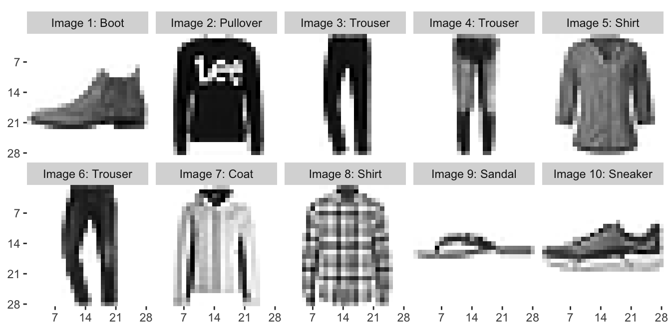
Before applying the KNN algorithm, the dataset was preprocessed by reshaping the images from 3D arrays to 2D arrays and flattening them into 784-dimensional vectors. The representation of all images can be seen as below:

A Single Sample

All Classes

Pixel Intensity Distribution

Random Samples

Class Distribution

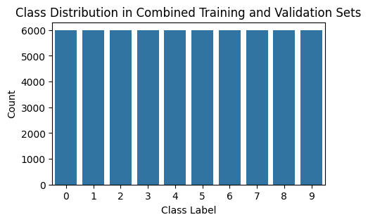
Even though the official dataset has stated that all classes have the same number of samples, let's see their distribution to double check.

Hyperparameter Tuning

The optimal value for the number of neighbors k in KNN was determined through experimentation, with values ranging from [1, 3, 7, 12, 20, 30, 50, 75, 100]. The performance of each configuration was evaluated on a validation set, and the optimal k value was selected based on the highest validation accuracy. $$k \in [1, 3, 7, 12, 20, 30, 50, 75, 100]$$

Also, different measure distances were utilized to retrain the classifier, which were:

Manhattan Distance (link)
Euclidean Distance (link)
Minkowski Distance (link)

The general formula for all of these distance measures is: $$D \left( x, y \right) = \left( \sum_{i=1}^{n} | x_{i} - x_{i} | ^{p} \right) ^{1/p}$$

Where:

$x$ and $y$ are the points we have as a pair to calculate their distance, and $x_i, y_i$ the data at the $i$-th dimension
$n$ is the total number of dimensions
$p$ is a positive real number, which determines the order of the Minkowski distance
if $p=1$ then we have Manhattan and if $p=2$ then we have Euclidean distance

Model Evaluation

The final KNN model was trained using the optimal k value determined during hyperparameter tuning. Its performance was assessed on a separate test set, and the results, including accuracy and a confusion matrix, are provided below.

k	1	3	7	12	20	30	50	75	100
Accuracy (%)	85.05	85.625	85.86	85.33	84.72	84.34	83.51	82.81	81.92

Confusion Matrix

Confusion Matrix
[[857   1  20  17   5   0  92   1   7   0]
 [  8 967   6  12   4   0   2   0   1   0]
 [ 20   2 814  11  78   0  75   0   0   0]
 [ 35   5  16 869  36   0  37   0   2   0]
 [  2   0 122  25 760   0  89   0   2   0]
 [  1   0   0   0   0 806   5 107   1  80]
 [173   0 129  23  74   0 588   0  13   0]
 [  0   0   0   0   0   2   0 957   0  41]
 [  1   1  13   5   7   0  12   7 952   2]
 [  0   0   0   0   0   1   1  28   0 970]]

Insights

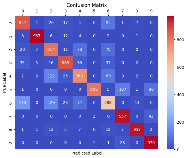
Before diving deep into the insights, I shall provide the name of each class to prevent any confusions:

T-shirt/top
Trouser
Pullover
Dress
Coat
Sandal
Shirt
Sneaker
Bag
Ankle boot

Diagonal Elements (True Positives)

The main diagonal of the matrix (from top-left to bottom-right) represents the number of correctly classified instances for each class. Higher values on the diagonal are desirable. As we can see, for classes 1, 7, 8, 9 we are getting values well above 90%. This means that these clothing items have been classified very accurately. The lowest belongs to class 6 with an accuracy of 58.8%, which is still better than randomly guessing but perhaps not as high as we wanted it to be. For example, class 3 also has a fairly high prediction rate.

Off-Diagonal Elements (Misclassifications)

Off-diagonal elements represent misclassifications. Higher values in off-diagonal elements indicate frequent misclassifications. For example, the prediction for class 0 with a true label of 6 has happened 173 times, which means that the model has falsely thought that the clothing item from class 0 is actually from class 6, which makes sense once you see these two classes correspond to "T-shirt/top" and "Shirt" respectively.

Class-wise Accuracy

Besides the classes 4, 6, the rest have been predicted with a high accuracy. Class 4 has been predicted with a rate of 76%, which is not low, but could be better. This class was seen similar to classes 2, 6 by the classifier the most, as "Pullover" and "Shirt" classes have good resemblence to "Coat".

Common Misclassifications

In the eye of the classifier, a few misclassifications were somewhat common:

misclassifying T-shirt/tops with Shirts
misclassifying Pullovers with Coats and Shirts

Strong Predictions

For classes "Trouser", "Bag" and "Anke Boot" classes, the model did an amazing job and only had few misclassifications. This might have to do with how unique these clothing items look and how much they differ from other classes in terms of their overall shapes and sizes.

Something Strange

Interestingly enough, the model did not misclassify class 7 with 5 that much (only 2 instances). However, it did wrongly predict class 5 as 7 quite a number of times, 107 times actually. So it's interesting to see that the classifier thought sandals look like sneakers while it avoided treating sneakers as sandals. One would think the misclassification should go both ways, as we have seen with the shirts and T-shirts example, or the pullovers with the coats instances.

Classification Report

Classification Report:
               precision    recall  f1-score   support

           0       0.78      0.86      0.82      1000
           1       0.99      0.97      0.98      1000
           2       0.73      0.81      0.77      1000
           3       0.90      0.87      0.89      1000
           4       0.79      0.76      0.77      1000
           5       1.00      0.81      0.89      1000
           6       0.65      0.59      0.62      1000
           7       0.87      0.96      0.91      1000
           8       0.97      0.95      0.96      1000
           9       0.89      0.97      0.93      1000

    accuracy                           0.85     10000
   macro avg       0.86      0.85      0.85     10000
weighted avg       0.86      0.85      0.85     10000

Min-Max Normalization and PCA

By applying Min-Max Normalization to the features (for rescaling) and Principal Component Analysis (PCA) for dimensionality reduction, we get an accuracy score of 85.09%. However, the accuracy seems to drop below what we achieved k=7, which was 85.40%. Therefore, this technique was not proven to be helpful.

Different Distance Measures

The original max prediction was with $k=7$ and the "Euclidean" distance measure, or $p=2$ in the KNeighborsClassifier(n_neighbors=k_value, p=2) line. By changing p to 1 and 3, we can get Manhattan and Minkowski (for p=3) predictions, which are as follows:

Test Accuracy with Manhattan distance: 0.8486
Test Accuracy with Minkowski distance (p=3): 0.8463

Meaning that we got 84.86% for Manhattan and 84.63% for Minkowski distance measures, which are both less than our original prediction score.

Future Work

While KNN has been the focus thus far, future iterations of this project may explore other machine learning algorithms, including deep learning approaches, to further enhance image classification performance.

Feel free to contribute or provide feedback on this project!

kouroshksh / fashion-mnist-classifier Goto Github PK