kovenda/a-b-testing-a-cotton-mill

To increase efficiency of a cotton mill. I set up an ANOVA 3 factor analysis model in R to determine best spindle & position that produces the longest roving. The only significant difference in roving length was observed when position was 3 and spindle was 1 or 2. (ANOVA Model in R)

A-B-Testing-a-Cotton-Mill

To increase efficiency of a cotton mill. I set up an ANOVA 3 factor analysis in R to determine best spindle & position that produces the longest roving. The only significant difference in roving length was observed when position was 3 and spindle was 1 or 2

Data

• Roving measurements of cotton in a mill, obtained on 4 days, from 4 spindles, at each of 3 positions. Presumably day and spindle would be random effects where as the position is fixed.
• The response variable is the Roving measurement. The factors are days, spindles, and positions.

Day	Spindle	Position	Measurment
1	4	2	382
3	2	1	401

Estimating the signficance of the main effects:

ggplot(Cotton, aes(x=as.factor(Day), y=Measurment)) + 
  geom_boxplot()
ggplot(Cotton, aes(x=as.factor(Spindle), y=Measurment)) + 
  geom_boxplot()
ggplot(Cotton, aes(x=as.factor(Position), y=Measurment)) + 
  geom_boxplot()

1. The plots show that the response variable, Measurement has constant variance.
2. Estimating the significance of the main effect Day: For the main effect Day to be significant the equation mean(Day 1) = mean (Day 2) =….= mean (Day 4) … = 0, has to be false, suggesting that at least one of the means of the Days is significantly different from another mean of Day. From the boxplot of Measurement vs Day, it is noticeable that all the mean Measurements over the four Days range from approximately 385 to 395 units of measurements. This 10 unit range is extremely narrow considering that the individual values have a 50 unit range from 370 to 420 units of measurement. Using the ratios of the ranges it is safe to estimate the chance of one day’s measurement mean to be significantly different from another day’s to be 1/5. With such a low chance of having a significant difference between the means of it’s levels I estimate the Day main effect to be insignificant.
3. Estimating the significance of the main effect Spindle: For the main effect Spindle to be significant the equation mean(Spindle 1) = mean (Spindle 2)=… = mean (Spindle 4) … = 0, has to be false, suggesting that at least one of the means of the Spindles is significantly from another mean of Spindle. From the boxplot of Measurement vs Spindle, it is noticeable that all the mean Measurements over the four Spindles range from approximately 385 to 395 units of measurements. This 10 unit range is extremly narrow considering that the individual values have a 50 unit range from 370 to 420 units of measurement. Using the ratios of the ranges it is safe to estimate the chance of one Spindle’s measurement mean to be significantly different from another Spindle’s to be 1/5. With such a low chance of having a significant difference between the means of it’s levels I estimate Spindle main effect to be insignificant.
4. Estimating the significance of the main effect Position: For the main effect Position to be significant the equation mean(Position 1) = mean (Position 2) = mean (Position 3) … = 0, has to be false, suggesting that at least one of the means of the Positions is significantly from another mean of Position. From the boxplot of Measurement vs Position, it is noticeable that all the mean Measurements over the three Positions range from approximately 388 to 395 units of meausurements. Since this is the smallest link of all the plots, I estimate Position main effect to be insignificant.

Estimating the Significance of interaction effect between Position and Day:

qplot (Day, Measurment, data=Cotton, color=as.factor(Position)) + stat_summary (fun=mean, geom="line") +
  facet_wrap (vars(Spindle), labeller="label_both")

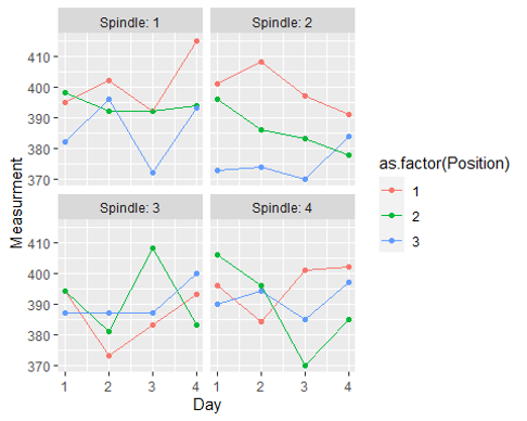
1. We look at the interaction between Position and Day adjusted for Spindle:
2. Our goal with this analysis is to estimate from the plot the existence of or the lack of a significant interaction between the measurement at each Position and Day by looking at the crossing of the levels of Position over the four days for each Spindle.
3. There exists a significant interaction between Position and Day when Spindle is 1 and 4; This significant interaction is estimable from the plot because the levels of Position are clearly crossing over the four days. There is however an ambiguity on the existence of a significant interaction between Position and Day when the Spindle is 3; Although the plot for when the Spindle is 3 shows some crossing of the levels of Position over the four days, it is difficult to say with certainty that the levels of Position are not parallel when you look at them from day to day, hence even though there exists some crossing, it is not enough to make the interaction significant. When spindle is 2, there is clear display of no interaction (or at least no significant interaction/ sufficient crossing of lines) between Position and Day as the levels of Position are clearly parallel to each other (at least for Days 1 to 3, even though Position 3 and 2 cross in Day 4).
4. Overall from the analysis we see that interaction between the measurement at each Position and Day by looking at the crossing of the levels of Position over the four days for each Spindle has 50% chance of being significant as it is significant when Spindle is 1 and 4 and not when the spindle is 2 and 3.

The following is an interaction plot between Position and Day:

qplot (Day, Measurment, data=Cotton, color=as.factor(Position)) + stat_summary (fun=mean, geom="line")
qplot (Day, Measurment, data=Cotton, color=as.factor(Spindle)) + stat_summary (fun=mean, geom="line") +
  facet_wrap (vars(Position), labeller="label_both")

The interaction shows a significant non-parallel effect between the levels of Position moving from day 1 to day 2. However there is no other significant non-parallel effects the levels of Position moving from one day to another. The final estimate for the interaction between Position and Day is that it is 1/3 significant.

• We look at the interaction between Spindle and Day adjusted for Position:

• Our goal with with this analysis is to estimate from the plot the existence of or the lack of a significant interaction between the measurement at each Spindle and Day by looking at the crossing of the levels of spindle over the four days for each Position.
• There exists a significant interaction between Spindle and Day at exh levels of position from one day to the other. This significant interaction is somehow estimable from the plot because the levels of Position are clearly crossing over on some of the days.
• Although the plot for when the Spindle is 3 shows some crossing of the levels of Position over the four days, it is difficult to say with certainty that the levels of Spindle are not parallel when you look at them from day to day, hence even though there exists some crossing, it is not enough to make the interaction significant. When Position is 2, there is clear display of no interaction (or at least no significant interaction/ sufficient crossing of lines) between Spindle and Day as the levels of Spindle are clearly parallel to each other (at least for Days 1 to 2, even though all four Spindles cross from day 3 to 4).
• Overall from the analysis we see that the interaction between the measurement at each Position and Day by looking at the crossing of the levels of Spindle over the four days for each Spindle has approximately 30% chance of being significant as it is significant in different levels of Position bot for specific days.

The interaction between Spindle and Day adjusted for Position:

qplot (Day, Measurment, data=Cotton, color=as.factor(Spindle)) + stat_summary (fun=mean, geom="line")

The interaction shows a significant non-parallel effect between the levels of 1 and 3 Spindle across the four days. However the Spindle 2 and 4 are not significant as they are close to parallel there is no other significant non-parallel effects the levels of Position moving from one day to another. The final estimate for the interaction between Spindle and Day is that it is 1/3 significant.

Fit the ANOVA model

cotton1 = aov (Measurment ~ factor(Position)*factor(Day)*factor(Spindle) - factor(Position):factor(Day):factor(Spindle), data=Cotton)
summary (cotton1)
# Model R-Squared
Rsquared_cotton1 = summary (lm (Measurment ~ Position*Day*Spindle, data=Cotton))$adj.r.squared
Rsquared_cotton1

• The fitted ANOVA model only has one significant main effect. The significant main effect is Position with a p-value well below the cut-off value of 0.05 at 0.0120. We thus reject the null hypothesis for the Position factor which states that mean(Position 1) = mean (Position 2) = mean (Position 3) … = 0, and we are therefore left to conclude that at least one mean (Position x) is different from at least another mean (Position x). This is conclusion is contradictory to our earlier estimate where we predicted the main effect Position to be insignificant. Furthermore the model has one marginally insignificant interaction effect. The marginally insignificant interaction effect is between Position and Spindle it has a p-value of 0.0577. The adjusted r-squared shows that our fitted ANOVA model explains only 9.34 % of the variation in our response variable roving measurements of cotton in a mill.

Model Evaluation (1. residual vs fitted plot 2. Normal Q-Q plot 3. scale location plot)

plot (cotton1, which = 1:3)

1. We can see from the residual vs fitted plot that the residuals seem to have an increasing variance from the left towards the right. However when one considers point 35 and you look at the red line (which approximately flat out) we see that the residuals do have constant variance.
2. The Normal Q-Q plot shows that the residuals do follow a normal distribution. All the residuals do fall between the expected range of -3 to 3 with some points like 35, 34 & 32 deviating from the line.
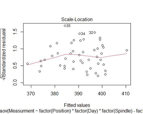
3. The scale location plot does show a slide increase in the residual variance but flattens off very quickly, therefore confirming our analysis that the residuals do have constant variance.

Response Transformation Analysis

Power Transformation from Boxcox:

MASS::boxcox (cotton1)

The Box Cox plot suggests that any power less than or equal to -2 will work as a response transformation. However it’s crucial to mention that the boxcox transformation suggested power has a pretty high 95% confidence interval which ranges from approximately -2 to everything less than -2. All though this confidence interval is very wide it is however significant as it does not include 0.

Power Transformation from log.sd vs log.mean:

Diam.summ = Cotton %>% group_by (Day) %>% summarise (mean.Measurment = mean (Measurment),
                                                     sd.Measurment = sd (Measurment))
Diam.summ$log.mean = log10 (Diam.summ$mean.Measurment)
Diam.summ$log.sd   = log10 (Diam.summ$sd.Measurment)
plot ( log.sd ~ log.mean, data=Diam.summ)
fit0 = lm ( log.sd ~ log.mean, data=Diam.summ)
abline (fit0)
summary(fit0)
confint (fit0)

The slope of log.sd vs log.mean is -15.988. To obtain the suggested power transformation for the response variable we need to subtract it from 1. However this slope has a 95% confidence interval that ranges from -39.63713 to 7.661716. Even though this confidence interval is just as wide as the confidence interval for the suggested power transformation from the boxcox plot, this one however includes zero and it is therefore not significant. Therefore because this response power transformation suggestion is not significant we will use the boxcox response power transformation.

Second Order model with response transfomation:

transformed_measurement = ((Measurment^(-2))/(-2))
cotton2 = aov (transformed_measurement ~ factor(Position)*factor(Day)*factor(Spindle) - factor(Position):factor(Day):factor(Spindle), data=Cotton)
Rsquared_cotton2 = summary (lm (transformed_measurement ~ Position*Day*Spindle, data=Cotton))$adj.r.squared
summary (cotton2)
Rsquared_cotton2

In the first order model where the response was not transformed the adjusted r-squared 0.09343949 and the only main effect that was significant was Position with a p-value of 0.0120 and a marginally insignificant interaction effect is between Day and Spindle it has a p-value of 0.0577. The second order transformed model is not that different from the first order untransformed model as it has an adjusted r-squared of 0.09007195 and the same significant main effect. However even though the adjusted r-square for this second order model is lower than the first order model with 0.003439, it has the interaction effect between Spindle and Position as significant with a p-value of 0.0462.

Model Evaluation (1. residual vs fitted plot 2. Normal Q-Q plot 3. scale location plot)

plot (cotton2, which = 1:3)

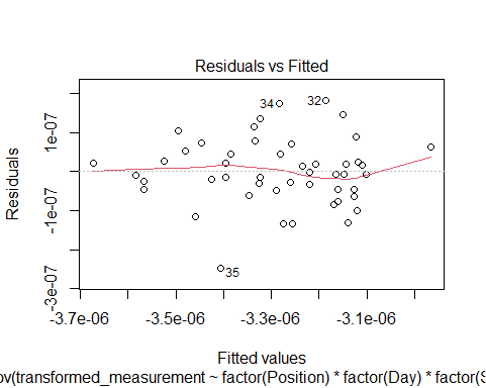
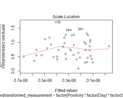
The residual plots remain unchnaged and still shows marginal constant variance and residuals following a normal distribution.

Analysing the significant main effect, Position:

summary (emmeans (cotton2, pairwise ~ Position), infer=c(T,T))
emmip (cotton2, Position ~ as.factor(Day))

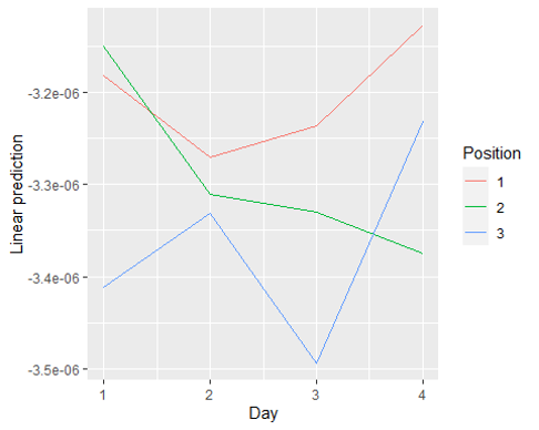
The position main effect is significant because level 1 of position is significantly higher than level 3 with a p-value of 0.0089.

Analysing the significant interaction effect between Position and Spindle:

cld(emmeans (cotton2, ~ Position|Spindle), Letters=LETTERS)
emmip (cotton2, Position ~ as.factor(Spindle))

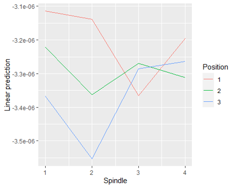
We see that when we adjust for Spindle the significant difference between the levels of position are as follows: The only significant difference between the levels of Position can only be observed when Spindle is 1 and 2. When Spindle is 1, level 3 and 1 of Position are significantly different from each. And when Spindle is 2, level 3 and 1 are significantly different from each other.

cld(emmeans (cotton2, ~ Spindle|Position), Letters=LETTERS)
emmip (cotton2, Spindle ~ as.factor(Position))

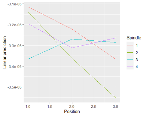
We see that when we adjust for Position the signficant difference between the levels of Spindle are as follows: The only significant difference between the levels of Spindle can only be observed when Position is 3. When Position is 3, level 4 and 1 of Spindle are significantly different from each.