legolason/pyqsofit

A code to fit the spectrum of quasar

pyqsofit's Issues

Fe_FWHM

I need to have a lower FWHM for the Fe_op. However even if I have a lower initial guess in the end I get something as high as >9000. If I change it in the code and instead of Fe_FWHM = pp[1] I have Fe_FWHM = 2000, I get better results but I am not sure if something like this it's possible without changing the code. I.e. to keep the Fe_FWHM low.

Fitting an emission line with multiple gaussians

Hello,
Is it possible to fit a single emission line using multiple gaussian curves, and if so, how? For example, if I have a quasar spectrum with a skewed broad HBeta line, is there some way to use two or three (or more) gaussian curves when fitting that specific line? Any help is greatly appreciated!

Spectral resolution

Hi again,

I use PyQSOfit to model the spectra of non-SDSS spectra. Is there a way to inform the code for the lower resolutions?

Thanks,

Lydia

q.err clarification

Hi again,

I want to clarify what is the return of q.err as I am a bit lost from the code.

Thanks,

Lydia

FeII plot line

Hi,

In the code the iron is plotted like that:

ax.plot(wave, f_conti_model, 'c', lw=2, label='FeII', zorder=7)

Is this correct? I had the idea that f_conti_model is the total continuum. Or we mean that it includes and the FeII?

Lydia

Runtime error

I git cloned the latest version and I am getting this error that as it seems PyQSOFit.py is missing the import of units package from astropy.

Lydia

Confirmation about luminosity

Just to confirm that the L5100 mentioned is λLλ(5100) which means erg/s.

Lydia

tie_width - multiple components

Hi,

When I have a two components broad Beta profile, is it possible to tie the width of another line to one of the components (i.e. the "less" broad one)?

Thanks,
Lydia

Inconsistent centerwave values stored in MCMC gauss results

Hi,

So I was going through your example.ipynb notebook and realized that the code is saving inconsistent centerwave values from the MCMC runs. Consider the following code excerpt from the example.ipynb

# Gaussian fitting results
print(q_mcmc.gauss_result_name)
print('')
print(q_mcmc.gauss_result)

['Hb_br_1_scale' 'Hb_br_1_scale_err' 'Hb_br_1_centerwave'
'Hb_br_1_centerwave_err' 'Hb_br_1_sigma' 'Hb_br_1_sigma_err'
'Hb_na_1_scale' 'Hb_na_1_scale_err' 'Hb_na_1_centerwave'
'Hb_na_1_centerwave_err' 'Hb_na_1_sigma' 'Hb_na_1_sigma_err'
'OIII4959c_1_scale' 'OIII4959c_1_scale_err' 'OIII4959c_1_centerwave'
'OIII4959c_1_centerwave_err' 'OIII4959c_1_sigma' 'OIII4959c_1_sigma_err'
'OIII5007c_1_scale' 'OIII5007c_1_scale_err' 'OIII5007c_1_centerwave'
'OIII5007c_1_centerwave_err' 'OIII5007c_1_sigma' 'OIII5007c_1_sigma_err'
'Ha_br_1_scale' 'Ha_br_1_scale_err' 'Ha_br_1_centerwave'
'Ha_br_1_centerwave_err' 'Ha_br_1_sigma' 'Ha_br_1_sigma_err'
'Ha_br_2_scale' 'Ha_br_2_scale_err' 'Ha_br_2_centerwave'
'Ha_br_2_centerwave_err' 'Ha_br_2_sigma' 'Ha_br_2_sigma_err'
'Ha_na_1_scale' 'Ha_na_1_scale_err' 'Ha_na_1_centerwave'
'Ha_na_1_centerwave_err' 'Ha_na_1_sigma' 'Ha_na_1_sigma_err'
'NII6549_1_scale' 'NII6549_1_scale_err' 'NII6549_1_centerwave'
'NII6549_1_centerwave_err' 'NII6549_1_sigma' 'NII6549_1_sigma_err'
'NII6585_1_scale' 'NII6585_1_scale_err' 'NII6585_1_centerwave'
'NII6585_1_centerwave_err' 'NII6585_1_sigma' 'NII6585_1_sigma_err'
'SII6718_1_scale' 'SII6718_1_scale_err' 'SII6718_1_centerwave'
'SII6718_1_centerwave_err' 'SII6718_1_sigma' 'SII6718_1_sigma_err'
'SII6732_1_scale' 'SII6732_1_scale_err' 'SII6732_1_centerwave'
'SII6732_1_centerwave_err' 'SII6732_1_sigma' 'SII6732_1_sigma_err']

[8.68700334e+00 1.01637686e-01 8.49006529e+00 7.91055207e-05
1.09929430e-02 1.31386254e-04 9.52499024e+00 1.37756743e-01
8.48916087e+00 2.22127131e-06 8.50657601e-04 4.75593423e-06
2.74390660e+01 4.17602049e-01 8.50903639e+00 0.00000000e+00
8.50657601e-04 0.00000000e+00 8.00441508e+01 3.85885690e-01
8.51865515e+00 0.00000000e+00 8.50657601e-04 0.00000000e+00
1.91934668e+01 4.09055820e-01 8.79087299e+00 5.83734285e-05
4.94704967e-03 4.57227276e-05 1.71879050e+01 6.54182588e-01
8.78853464e+00 9.25178445e-05 1.02397215e-02 7.73149317e-05
2.32468583e+01 1.73300314e-01 8.78925565e+00 5.30076034e-06
6.98470792e-04 8.59528736e-06 1.08016573e+01 6.24946073e-02
8.78700402e+00 0.00000000e+00 6.98470792e-04 0.00000000e+00
3.24049720e+01 0.00000000e+00 8.79239896e+00 0.00000000e+00
6.98470792e-04 0.00000000e+00 1.16004933e+01 8.31017257e-02
8.81239560e+00 0.00000000e+00 6.98470792e-04 0.00000000e+00
1.16004933e+01 0.00000000e+00 8.81453374e+00 0.00000000e+00
6.98470792e-04 0.00000000e+00]

# Gaussian fitting results
print(q_mcmc.gauss_result_name[::2])
print('')
print(q_mcmc.gauss_result_all)
print(np.shape(q_mcmc.gauss_result_all))

['Hb_br_1_scale' 'Hb_br_1_centerwave' 'Hb_br_1_sigma' 'Hb_na_1_scale'
'Hb_na_1_centerwave' 'Hb_na_1_sigma' 'OIII4959c_1_scale'
'OIII4959c_1_centerwave' 'OIII4959c_1_sigma' 'OIII5007c_1_scale'
'OIII5007c_1_centerwave' 'OIII5007c_1_sigma' 'Ha_br_1_scale'
'Ha_br_1_centerwave' 'Ha_br_1_sigma' 'Ha_br_2_scale' 'Ha_br_2_centerwave'
'Ha_br_2_sigma' 'Ha_na_1_scale' 'Ha_na_1_centerwave' 'Ha_na_1_sigma'
'NII6549_1_scale' 'NII6549_1_centerwave' 'NII6549_1_sigma'
'NII6585_1_scale' 'NII6585_1_centerwave' 'NII6585_1_sigma'
'SII6718_1_scale' 'SII6718_1_centerwave' 'SII6718_1_sigma'
'SII6732_1_scale' 'SII6732_1_centerwave' 'SII6732_1_sigma']

[[ 7.85981471e+00 9.70211243e-04 1.22709280e-02 ... 1.16004933e+01
-1.93092932e-04 6.98470792e-04]
[ 8.47034947e+00 6.09780117e-04 1.09293111e-02 ... 1.16004933e+01
-1.93092932e-04 6.98470792e-04]
[ 7.77712590e+00 1.57125188e-03 1.19115053e-02 ... 1.16004933e+01
-1.93092932e-04 6.98470792e-04]
...
[ 8.08952745e+00 1.46338017e-03 1.19396797e-02 ... 1.16004933e+01
-1.93092932e-04 6.98470792e-04]
[ 8.18530017e+00 7.33854121e-04 1.16541468e-02 ... 1.16004933e+01
-1.93092932e-04 6.98470792e-04]
[ 8.52164429e+00 3.60590882e-04 1.09389864e-02 ... 1.16004933e+01
-1.93092932e-04 6.98470792e-04]]
(1000, 33)

As you can see, for example, the Hb_br_1_centerwave value stored in q_mcmc.gauss_result (8.49006529e+00) vs the values stored in q_mcmc.gauss_result_all (9.70211243e-04) are different orders of magnitudes. It would be great if you could take a look at this issue since it is important in order to calculate error values for each parameter for narrow lines particularly.

Thanks,
Rohan

Clarification of each line_prop calculation and results

Hi,

I am doing some fitting for several SDSS spectra and would like to understand the output results better.
I have performed some tests on the code and have read the code itself but I would like some clarification on how the FWHM is calculated in the results file, the FWHM returned from the function line_prop, and line_prop_from_name

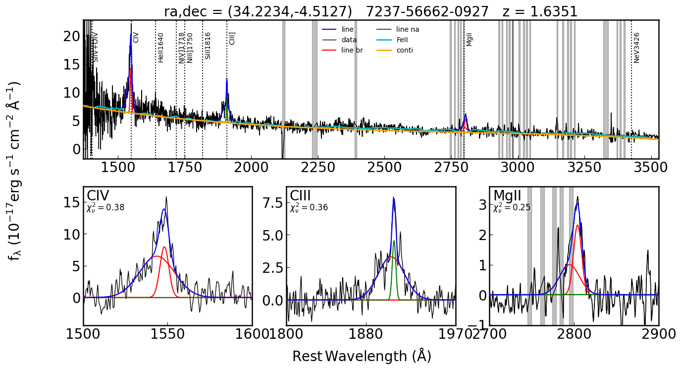
For context, I am fitting MgII lines with 1 narrow and 1 broad line as a baseline. As you can see, the MgII is fitted with 2 broad components instead. When I called line_prop_from_name('MgII_br', 'broad') I found that the results are inconsistent with the results MgII_whole_br_fwhm. however, I noticed that line_prop_from_name('MgII_nl', 'broad') also returns a non-zero value.
I tested the code assuming different numbers lines to fit in MgII (eg, only broad, only gaussian, etc).

I check the code and would like the following points.

1. My understanding now is that the FWHM of whole_br listed in the results file and stored under fur_result is calculated from the model emission line constructed from all broad line components in the best fit and calculated numerically following Peterson+04. Is this correct?
2. Internally, initially assumed narrow emission lines can be switched to broad emission lines if the line widths exceed a threshold (ln_sigma_br). Correct?
3. If the line with an assumed narrow line width (eg. MgII_nl) is switched into a broad line, it is added to the composite broad line into the final result file correct?
4. line_prop (and by extension line_prop_from_name) checks the best fit emission line width correct? eg. I noticed that line_prop_from_name('MgII_nl', 'broad') returns the result of the best fit suggesting it is broad.

Thanks for the work you guys have done btw! Sorry if the questions are a bit convoluted.

Issue with Determining Fit Parameters for Emission Lines

Hi,

I am having trouble understanding how to get the fit parameters for specific emission lines. Following the example in Step 5 for broad Hb:

fwhm,sigma,ew,peak,area = q.line_prop(q.linelist[6][0],q.line_result[12:15],'broad')
print("Broad Hb:")
print("FWHM (km/s)", np.round(fwhm,1))
print("Sigma (km/s)", np.round(sigma,1))
print("EW (A)",np.round(ew,1))
print("Peak (A)",np.round(peak,1))
print("area (10^(-17) erg/s/cm^2)",np.round(area,1))

I get the following error:

pp = pp.astype(float)
ValueError: could not convert string to float: 'Hb'

I have tried to look through the source code for any help in what I should be putting in as the second parameter for the line_prop() function and it seems like it should be the fit parameters, but I am unsure what I should be looking for in the line_result array. Any help for determining what I should be using in the line_result array as the fit parameters would be immensely appreciated!

Continuum fitting

I have an issue with continuum fitting and I wonder if you have come across this or can suggest a solution. When I fit the continuum for the full spectrum with simply the power-law it doesn't fit very well on the red part. When I add a polynomial contribution it behaves weird. See attached files. Playing around with the initial guess doesn't change things. Let me know if you have any suggestion. Fitting the blue and the red spectrum separately can be a solution but I would like it if it was possible to fit the whole spectrum.

Approximate FWHM of the line

Hi,

Is there a way to calculate the "total" approximate FWHM for a line with multiple components using the code itself?

Is that the e.g. Hb_whole_br_fwhm in q.all_result?

Thanks,

Lydia

Error when Fe_uv_op set as False and MCMC=True

Hello,

Thanks for this great package. I just tried the latest version of PyQsoFit and attempted to estimate the uncertainties using the MCMC option. My input is as follows:

data = fits.open(os.path.join(path_ex, 'data/spec-2788-54553-0051.fits'))
lam = 10**data[1].data['loglam'] # OBS wavelength [A]
flux = data[1].data['flux'] # OBS flux [erg/s/cm^2/A]
err = 1/np.sqrt(data[1].data['ivar']) # 1 sigma error
z = data[2].data['z'][0] # Redshift

ra = data[0].header['plug_ra'] # RA
dec = data[0].header['plug_dec'] # DEC
plateid = data[0].header['plateid'] # SDSS plate ID
mjd = data[0].header['mjd'] # SDSS MJD
fiberid = data[0].header['fiberid'] # SDSS fiber ID

q = QSOFit(lam, flux, err, z, ra=ra, dec=dec, plateid=plateid, mjd=mjd, fiberid=fiberid, path=path_ex)

q.Fit(name=None, nsmooth=1, and_or_mask=False, deredden=True, reject_badpix=False, wave_range=None,
wave_mask=None, decompose_host=False, Mi=None, npca_gal=5, npca_qso=20,
Fe_uv_op=False, Fe_flux_range=None, poly=True, BC=False, rej_abs=False, linefit=True,
initial_guess=None,
MCMC=True, nburn=100, nsamp=200, nthin=10, epsilon_jitter=1e-5, plot_corner=True,
save_result=True, plot_fig=True, save_fig=True, plot_line_name=True, plot_legend=True,
save_fig_path=path_out, save_fits_path=path_out, save_fits_name=None)

This gives the following error:

File "new_pyqsofit.py", line 36, in
q.Fit(name=None, nsmooth=1, and_or_mask=False, deredden=True, reject_badpix=False, wave_range=None,
File "/opt/miniconda3/lib/python3.8/site-packages/PyQSOFit-1.2.0-py3.8.egg/pyqsofit/PyQSOFit.py", line 475, in Fit
self.fit_continuum(self.wave, self.flux, self.err, self.ra, self.dec, self.plateid, self.mjd, self.fiberid)
File "/opt/miniconda3/lib/python3.8/site-packages/PyQSOFit-1.2.0-py3.8.egg/pyqsofit/PyQSOFit.py", line 1230, in fit_continuum
Fe_flux_results = np.empty((len(samples), np.shape(self.Fe_flux_range.flatten())[0]//2))
AttributeError: 'NoneType' object has no attribute 'flatten'

I request you to kindly take a look at the problem.

Question:q.flux and q.line_flux

Hi,

Are q.flux and q.line_flux host or not host subtracted?

Thank you,

Lydia

decompsition-host

Dear Guo
Thank you for your code, it is really a useful tool. When i run the example, i select the parameter "decompose-host = True",it will back an error like the picture

and if i select "decompose-host = False" it will get a result but i do not believe it.
I am a beginner in python.this may be a silly question but i appreciate your help.
Thank you!

'_whole' broad lines calculation

Hi,

Could you briefly explain to me the method that it's used in the code to calculate the the 'whole' FWHM etc for line that have multiple broad components?

Lydia

Numpy attribute error

Hi,

I am looking to fit some spectra of AGN using pyQSOfit and ran in to an issue related to numpy attributes when testing the with the example. What is the working numpy version for pyQSOfit (also for other packages would be nice to know too.)

My package setup includes
numpy 1.20.0
scipy 1.6.0
astropy 5.1
PyAstronomy 0.18.0
Sfdmap 0.1.1
kapteyn 3.0
python 3.8

I know that the running version is python 3.6 and I will check with that in a bit. I'm opening the ticket since the current issue seem to be more related to numpy.

Cheers,

Klod

AttributeError Traceback (most recent call last)
in
4 start = timeit.default_timer()
5 # do the fitting
----> 6 q.Fit(name = None,nsmooth = 1, and_or_mask = False, deredden = True, reject_badpix = False, wave_range = None,
7 wave_mask =None, decomposition_host = True, Mi = None, npca_gal = 5, npca_qso = 20,
8 Fe_uv_op = True, Fe_flux_range=np.array([4435,4685]), poly = True, BC = False, rej_abs = False,
~/ext_disk/disk_1/Dropbox/studies/Research/Data_reduction/WERGS/data_anal/specfit/WERGS_2021/HSC_42045337531063074/PyQSOFit-master/example/../pyqsofit/PyQSOFit.py in Fit(self, name, nsmooth, and_or_mask, reject_badpix, deredden, wave_range, wave_mask, decomposition_host, BC03, Mi, npca_gal, npca_qso, Fe_uv_op, Fe_flux_range, poly, BC, rej_abs, initial_guess, MC, n_trails, linefit, tie_lambda, tie_width, tie_flux_1, tie_flux_2, save_result, plot_fig, save_fig, plot_line_name, plot_legend, dustmap_path, save_fig_path, save_fits_path, save_fits_name)
405 if linefit == True:
406
--> 407 self._DoLineFit(self.wave, self.line_flux, self.err, self.conti_fit)
408 else:
409 self.ncomp = 0
~/ext_disk/disk_1/Dropbox/studies/Research/Data_reduction/WERGS/data_anal/specfit/WERGS_2021/HSC_42045337531063074/PyQSOFit-master/example/../pyqsofit/PyQSOFit.py in _DoLineFit(self, wave, line_flux, err, f)
910 for ii in range(ncomp):
911 compcenter = allcompcenter[ii]
--> 912 ind_line = np.where(linelist['compname'] == uniq_linecomp_sort[ii], True, False) # get line index
913 nline_fit = np.sum(ind_line) # n line in one complex
914 linelist_fit = linelist[ind_line]
~/.local/lib/python3.8/site-packages/pyfits/py3compat.py in getitem(self, obj)
101 if isinstance(val, numpy.character):
102 temp = val.rstrip()
--> 103 if numpy.char._len(temp) == 0:
104 val = ''
105 else:
AttributeError: module 'numpy.core.defchararray' has no attribute '_len'

Calculation of "whole"

Hi,

If I have two broad components for a different line (other than the standard Balmer lines), is there a way to calculate the whole FWHM, etc using some function from the code?

Thanks,

Lydia

Pl Slope problem

Code is giving opposite slopes for the two different spectrums of a similar source. What can be the possible reason? Since the slope of the spectrum looks very similar. I have also tried to fit the spectrum in a particular range but still the problem persists.

Preferred Citation in ReadMe

I see that you have created an ASCL identifier for this code; I also note that your code is being mentioned in manuscripts submitted to the AAS Journals.

I ask that you please list the preferred citation for your code in the main ReadMe file for this repository. If that citation is the ASCL identifier then it should read something like:

The preferred citation for this code is Guo, Shen & Wang (2018), ascl:1809:008
@misc{2018ascl.soft09008G,
author = {{Guo}, H. and {Shen}, Y. and {Wang}, S.},
title = "{PyQSOFit: Python code to fit the spectrum of quasars}",
keywords = {Software },
howpublished = {Astrophysics Source Code Library},
year = 2018,
month = sep,
archivePrefix = "ascl",
eprint = {1809.008},
adsurl = {http://adsabs.harvard.edu/abs/2018ascl.soft09008G},
adsnote = {Provided by the SAO/NASA Astrophysics Data System}
}

Lastly, it would be good to document in this ReadMe the relationship between this code and other versions of the QSO fitting algorithms presented here.

August Muench
Data Editor, AAS Journals.

Error using code on Google Colab

Hello,

I'm trying to replicate your example code (from example.ipynb), but I'm getting an error with some of the paths.

---------------------------------------------------------------------------
FileNotFoundError                         Traceback (most recent call last)
<ipython-input-10-bd3ae4a2d819> in <module>()
      1 start = timeit.default_timer()
      2 # do the fitting
----> 3 q.Fit(name = None,nsmooth = 1, and_or_mask = False, deredden = True, reject_badpix = False, wave_range = None,      wave_mask =None, decomposition_host = True, Mi = None, npca_gal = 5, npca_qso = 20,       Fe_uv_op = True, poly = True, BC = False, rej_abs = False, initial_guess = None, MC = False,       n_trails = 5, linefit = True, tie_lambda = True, tie_width = True, tie_flux_1 = True, tie_flux_2 = True,      save_result = True, plot_fig �...
      4 
      5 end = timeit.default_timer()

9 frames
/usr/local/lib/python3.6/dist-packages/astropy/io/fits/util.py in fileobj_open(filename, mode)
    394     """
    395 
--> 396     return open(filename, mode, buffering=0)
    397 
    398 

FileNotFoundError: [Errno 2] No such file or directory: '.pca/Yip_pca_templates/gal_eigenspec_Yip2004.fits'

I'm sharing the notebook as I'm using it (with all the corresponding installations), so you can replicate the problem: https://colab.research.google.com/drive/1izwfcMRtefhgK_FuDf29fVwRshOPQyFg?usp=sharing

not correct error Galactic extinction

PyQSOFit/PyQSOFit.py

Line 600 in 5ef93a3

def _DeRedden(self,lam,flux,ra,dec,dustmap_path):

Velocity offset

Hi,

When we have a velocity offset of 0.01, does this mean we allow of an offset of 7000km/s(!)?

Thanks,

Lydia

Question about the calculation of EW

Thanks for your excellent code and I've used it for nearly a year recommended by my tutor. I never use the EW data from this code before however, I find that the EW data from most of my fitting results are 'inf'. And recently, I find that in line 1274 of PyQSOFit.py, where the EW is calculated, the calculation seems not correct.

     #-----line properties calculation function--------
    def line_prop(self,compcenter,pp,linetype):
        """
        Calculate the further results for the broad component in emission lines, e.g., FWHM, sigma, peak, line flux
        The compcenter is the theortical vacuum wavelength for the broad compoenet.
        """
        pp = pp.astype(float)
        if linetype == 'broad':
            ind_br = np.repeat(np.where(pp[2::3] > 0.0017,True,False),3)
           
        elif linetype == 'narrow':
            ind_br = np.repeat(np.where(pp[2::3] < 0.0017,True,False),3)
            
        else:
            raise RuntimeError("line type should be 'broad' or 'narrow'!")
            
                
        ind_br[9:] = False # to exclude the broad OIII and broad He II
        
        p = pp[ind_br]
        del pp 
        pp = p


        c = 299792.458 # km/s
        n_gauss = int(len(pp)/3)
        if n_gauss == 0:
            fwhm,sigma,ew,peak,area = 0.,0.,0.,0.,0.
        else:
            cen = np.zeros(n_gauss)
            sig = np.zeros(n_gauss)

            for i in range(n_gauss):
                cen[i] = pp[3*i+1]
                sig[i] = pp[3*i+2]


            #print cen,sig,area
            left = min(cen-3*sig)
            right = max(cen+3*sig)
            disp = 1.e-4
            npix = int((right-left)/disp)


            xx = np.linspace(left, right, npix)
            yy = manygauss(xx,pp)

            ff = interpolate.interp1d(np.log(self.wave),self.PL_poly_BC, bounds_error = False, fill_value = 0)
            contiflux = ff(xx)


            #find the line peak location
            ypeak = yy.max()
            ypeak_ind= np.argmax(yy)
            peak = np.exp(xx[ypeak_ind])

            #find the FWHM in km/s
            #take the broad line we focus and ignore other broad components such as [OIII], HeII


            if n_gauss > 3:
                spline = interpolate.UnivariateSpline(xx, manygauss(xx,pp[0:9])-np.max(manygauss(xx,pp[0:9]))/2, s = 0)
            else:
                spline = interpolate.UnivariateSpline(xx, yy-np.max(yy)/2, s = 0)
            if len(spline.roots()) > 0:
                fwhm_left, fwhm_right = spline.roots().min(), spline.roots().max()
                fwhm = abs(np.exp(fwhm_left)-np.exp(fwhm_right))/compcenter*c

                #calculate the total broad line flux
                area = (np.exp(xx)*yy*disp).sum()

                #calculate the line sigma and EW in normal wavelength
                lambda0 = 0.
                lambda1 = 0.
                lambda2 = 0.
                ew = 0
                for lm in range(npix):
                    lambda0 = lambda0 + manygauss(xx[lm],pp)*disp*np.exp(xx[lm])
                    lambda1 = lambda1 + np.exp(xx[lm])*manygauss(xx[lm],pp)*disp*np.exp(xx[lm])
                    lambda2 = lambda2 + np.exp(xx[lm])**2*manygauss(xx[lm],pp)*disp*np.exp(xx[lm])

                    ew = ew + abs(manygauss(xx[lm],pp)/contiflux[lm])*disp*np.exp(xx[lm])

                sigma = np.sqrt(lambda2/lambda0-(lambda1/lambda0)**2) / compcenter*c
            else:
                fwhm,sigma,ew,peak,area = 0.,0.,0.,0.,0.

        return fwhm,sigma,ew,peak,area

I'm not quite sure about this and I haven't compare your result with Shen's IDL code results. But as you can see the 'disp' is 1.e-4 which is the gap of wavelength in log10. This is defined by the 'loglam' in sdss fits file. However, the approximation of disp=log10(x_(i+1))-log10(x_i) is not dx/x_i. As far as I can see, it should like this:
ew = ew + abs(manygauss(xx[lm],pp)/contiflux[lm])*disp*np.exp(xx[lm])*np.log(10)
I just have some question about this part. I haven't read the whole code, so if I have any mistakes, please forgive me. Many thanks!

Power law

Hi,

Is it possible to not have a power law fitting for the continuum and only have the polynomial term?

Cheers,

Lydia

Question about tie_width.

My understanding is that tie_width is tying these with the same windex (third from end). However I have done it for three lines but the FWHM in the end is quite different for each line. Am I getting something wrong?

Thanks,

Lydia

Manygauss returns NaN

Hi,

First thanks a lot for the very well-written and easy-to-use code!

I have a problem while trying to fit a starforming galaxy (spec-1172-52759-0097). Although I've managed to fit kinda well the spectrum lines using for qsopar:

newdata = np.rec.array([(6564.61,'Ha',6400.,6800.,'Ha_br',3,5e-3,0.004,0.05,0.015,0,0,0,0.05),
(6564.61,'Ha',6400.,6800.,'Ha_na',1,1e-3,2e-4,0.0017,0.01,1,1,0,0.02),
(6549.85,'Ha',6400.,6800.,'NII6549',1,1e-3,2.3e-4,0.0017,5e-3,1,1,1,0.001),
(6585.28,'Ha',6400.,6800.,'NII6585',1,1e-3,2.3e-4,0.0017,5e-3,1,1,1,0.003),
(6718.29,'Ha',6400.,6800.,'SII6718',1,1e-3,2.3e-4,0.0017,5e-3,1,1,2,0.001),
(6732.67,'Ha',6400.,6800.,'SII6732',1,1e-3,2.3e-4,0.0017,5e-3,1,1,2,0.001),
(4862.68,'Hb',4640.,5100.,'Hb_br',1,5e-3,0.004,0.05,0.01,0,0,0,0.01),
(4862.68,'Hb',4640.,5100.,'Hb_na',1,0.5e-3,2.3e-4,0.0017,0.01,1,1,0,0.002),
(4960.30,'Hb',4640.,5100.,'OIII4959c',1,1e-3,2.3e-4,0.0017,0.01,1,1,0,0.002),
(5008.24,'Hb',4640.,5100.,'OIII5007c',1,1e-3,2.3e-4,0.0017,0.01,1,1,0,0.004),
(4960.30,'Hb',4640.,5100.,'OIII4959w',1,3e-3,2.3e-4,0.004,0.01,2,2,0,0.001),
(5008.24,'Hb',4640.,5100.,'OIII5007w',1,3e-3,2.3e-4,0.004,0.01,2,2,0,0.002),
#(4687.02,'Hb',4640.,5100.,'HeII4687_br',1,5e-3,0.004,0.05,0.005,0,0,0,0.001),
#(4687.02,'Hb',4640.,5100.,'HeII4687_na',1,1e-3,2.3e-4,0.0017,0.005,1,1,0,0.001),
#(3934.78,'CaII',3900.,3960.,'CaII3934',2,1e-3,3.333e-4,0.0017,0.01,99,0,0,-0.001),
#(3728.48,'OII',3650.,3800.,'OII3728',1,1e-3,3.333e-4,0.0017,0.01,1,1,0,0.001),
#(3426.84,'NeV',3380.,3480.,'NeV3426',1,1e-3,3.333e-4,0.0017,0.01,0,0,0,0.001),
#(3426.84,'NeV',3380.,3480.,'NeV3426_br',1,5e-3,0.0025,0.02,0.01,0,0,0,0.001),
],\

When I try to plot the different parts using the example:

fig=plt.figure(figsize=(15,8))
#plot the quasar rest frame spectrum after removed the host galaxy component
plt.plot(q.wave,q.flux,'grey')
plt.plot(q.wave,q.err,'r')

#To plot the whole model, we use Manygauss to reappear the line fitting results saved in gauss_result
plt.plot(q.wave,q.Manygauss(np.log(q.wave),q.gauss_result)+q.f_conti_model,'b',label='line',lw=2)
plt.plot(q.wave,q.f_conti_model,'c',lw=2)
plt.plot(q.wave,q.PL_poly,'orange',lw=2)
plt.plot(q.wave,q.host,'m',lw=2)

plt.xlim(3500,8000)
plt.xlabel(r'$\rm Rest , Wavelength$ ($\rm \AA$)',fontsize = 20)
plt.ylabel(r'$\rm f_{\lambda}$ ($\rm 10^{-17} erg;s^{-1};cm^{-2};\AA^{-1}$)',fontsize = 20)

I see that Manygauss (Onegauss as well) gives Nan. If you have any idea why this happens or you see any mistake in my code, please let me know!

Thanks,
Lydia

Continuum fitting

I have a question with regards to the continuum fitting. I can see that iron continuum fitting depends on the windows given. I wanted to know if at any point the power law, the polynomial or the iron-optical avoid the ranges in the lines parameter.

Thank you.

Lydia

Min/max sigma

Hi again,

I am kinda confused with the way the limits are set. E.g. if the limits in FWHM 2000-10000 km/s what's the correct numbers for qsopar? I am afraid that either I am doing something wrong (in trying to go from FWHM to sigma) or I have misunderstood something as my numbers are quite different.

Thanks,

Lydia

Fe complex persists even after disabling

Hello,

Thanks for this great package. I am trying to fit an SDSS spectrum using the latest code. My input is as follows:

import glob, os,sys,timeit
import matplotlib
import numpy as np
from pyqsofit.PyQSOFit import QSOFit
from astropy.io import fits
import matplotlib.pyplot as plt
import warnings
warnings.filterwarnings("ignore")
QSOFit.set_mpl_style()

data = fits.open(os.path.join(path_ex, 'data/spec-2788-54553-0051.fits'))
lam = 10**data[1].data['loglam'] # OBS wavelength [A]
flux = data[1].data['flux'] # OBS flux [erg/s/cm^2/A]
err = 1/np.sqrt(data[1].data['ivar']) # 1 sigma error
z = data[2].data['z'][0] # Redshift

ra = data[0].header['plug_ra'] # RA
dec = data[0].header['plug_dec'] # DEC
plateid = data[0].header['plateid'] # SDSS plate ID
mjd = data[0].header['mjd'] # SDSS MJD
fiberid = data[0].header['fiberid'] # SDSS fiber ID

q = QSOFit(lam, flux, err, z, ra=ra, dec=dec, plateid=plateid, mjd=mjd, fiberid=fiberid, path=path_ex)
q.Fit(name=None, nsmooth=1, and_or_mask=False, deredden=True, reject_badpix=False, wave_range=None,
wave_mask=None, decompose_host=False, Mi=None, npca_gal=5, npca_qso=20,
Fe_uv_op=False, Fe_flux_range=None, poly=True, BC=False, rej_abs=False, linefit=True,
initial_guess=None,
#MCMC=False, nburn=100, nsamp=200, nthin=10, epsilon_jitter=1e-5, plot_corner=True,
save_result=True, plot_fig=True, save_fig=True, plot_line_name=True, plot_legend=True,
save_fig_path=path_out, save_fits_path=path_out, save_fits_name=None)

This plots the following output:

As can be seen, even though I have disabled the Fe component, the code is still trying to fit it which leads to the poor fit of the [OII] line.

Interestingly, when I tried it with an older version of PyQsoFit, it did the job correctly:

It would be great if you could please take a look and let me know a possible remedy.

Line flux calculation

Hi,

I'm a newcomer in spectral line analysis and I got a question using your code. I noticed that you calculated the gaussian line flux by intergrating the area under the profile :

       if len(spline.roots()) > 0:
            fwhm_left, fwhm_right = spline.roots().min(), spline.roots().max()
            fwhm = abs(np.exp(fwhm_left)-np.exp(fwhm_right))/compcenter*c

            #calculate the total broad line flux
            area = (np.exp(xx)*yy*disp).sum()

For a gaussian profile, the area under it should equal the value of its scale (i,e. pp[0]), summing 'flux densitydisp' can get the consistant area. Could you please tell me why you using 'wavelengthflux densitydisp' instead of 'flux densitydisp'? Disp shoule have a unit of Angstrom so the unit of area is actually (erg/s/cm^2/A)AA ?

I'm confused here and Thank you in advance.

Underfitting emission lines

Hi,

I have been using PyQSOFit for fitting spectra of emission line galaxies and I've noticed that the code seems to underfit multiple emission lines in a spectrum quite often. An example fit is attached below. For reference these spectra are from the DEIMOS 10k catalog. Any suggestions on how to tackle this issue or what might be causing it?

Help: Fitting OIII and Hb emission lines using the code

Dear @legolason,

Thank you for the code. It is indeed very helpful and powerful tool. I have started using the code to fit the SDSS spectra, but focusing on the Hb and [OIII] lines. However, I am having challenges in fitting the lines. This may be a naive or silly question but I appreciate your help.

Basically I am only adding back the OIII wings in this part,
newdata = np.rec.array([(6564.61,'Ha',6400.,6800.,'Ha_br',3,5e-3,0.004,0.05,0.015,0,0,0,0.05),
(6564.61,'Ha',6400.,6800.,'Ha_na',1,1e-3,5e-4,0.0017,0.01,1,1,0,0.002),
(6549.85,'Ha',6400.,6800.,'NII6549',1,1e-3,2.3e-4,0.0017,5e-3,1,1,1,0.001),
(6585.28,'Ha',6400.,6800.,'NII6585',1,1e-3,2.3e-4,0.0017,5e-3,1,1,1,0.003),
(6718.29,'Ha',6400.,6800.,'SII6718',1,1e-3,2.3e-4,0.0017,5e-3,1,1,2,0.001),
(6732.67,'Ha',6400.,6800.,'SII6732',1,1e-3,2.3e-4,0.0017,5e-3,1,1,2,0.001),
(4862.68,'Hb',4640.,5100.,'Hb_br',1,5e-3,0.004,0.05,0.01,0,0,0,0.01),
(4862.68,'Hb',4640.,5100.,'Hb_na',1,1e-3,2.3e-4,0.0017,0.01,1,1,0,0.002),
(4960.30,'Hb',4640.,5100.,'OIII4959c',1,1e-3,2.3e-4,0.0017,0.01,1,1,0,0.002),
(5008.24,'Hb',4640.,5100.,'OIII5007c',1,1e-3,2.3e-4,0.0017,0.01,1,1,0,0.004),
(4960.30,'Hb',4640.,5100.,'OIII4959w',1,3e-3,2.3e-4,0.004,0.01,2,2,0,0.001),
(5008.24,'Hb',4640.,5100.,'OIII5007w',1,3e-3,2.3e-4,0.004,0.01,2,2,0,0.002),
(2798.75,'MgII',2700.,2900.,'MgII_br',1,5e-3,0.004,0.05,0.0017,0,0,0,0.05),
(2798.75,'MgII',2700.,2900.,'MgII_na',2,1e-3,5e-4,0.0017,0.01,1,1,0,0.002),
(1908.73,'CIII',1700.,1970.,'CIII_br',2,5e-3,0.004,0.05,0.015,99,0,0,0.01),
(1549.06,'CIV',1500.,1700.,'CIV_br',1,5e-3,0.004,0.05,0.015,0,0,0,0.05),
(1549.06,'CIV',1500.,1700.,'CIV_na',1,1e-3,5e-4,0.0017,0.01,1,1,0,0.002),
(1215.67,'Lya',1150.,1290.,'Lya_br',1,5e-3,0.004,0.05,0.02,0,0,0,0.05),
(1215.67,'Lya',1150.,1290.,'Lya_na',1,1e-3,5e-4,0.0017,0.01,0,0,0,0.002)\

And then the input is
q.Fit(name = None,nsmooth = 1, and_or_mask = False, deredden = True, reject_badpix = False, wave_range = None,
wave_mask =None, decomposition_host = True, Mi = None, npca_gal = 5, npca_qso = 20,
Fe_uv_op = True, Fe_flux_range=np.array([4435,4685]), poly = True, BC = False, rej_abs = False,
initial_guess = None, MC = 50, n_trails = 5, linefit = True, tie_lambda = True, tie_width = True,
tie_flux_1 = True, tie_flux_2 = True, save_result = True, plot_fig = True,save_fig = False,
plot_line_name = True, plot_legend = True, dustmap_path = path4, save_fig_path = path3,
save_fits_path = path2,save_fits_name = None)

And these are the result:
Input:
fwhm,sigma,ew,peak,area = q.line_prop(q.linelist[8][0],q.line_result[18:21],'narrow')
fwhm,sigma,ew,peak,area = q.line_prop(q.linelist[9][0],q.line_result[21:24],'narrow')
fwhm,sigma,ew,peak,area = q.line_prop(q.linelist[10][0],q.line_result[24:27],'broad')
fwhm,sigma,ew,peak,area = q.line_prop(q.linelist[11][0],q.line_result[27:30],'broad')
output:
Narrow [OIII]4959c:
FWHM (km/s) 613.1
Sigma (km/s) 254.9
EW (A) 94.2
Peak (A) 4958.9
area (10^(-17) erg/s/cm^2) 202.8
Narrow [OIII]5007c:
FWHM (km/s) 613.1
Sigma (km/s) 254.9
EW (A) 276.7
Peak (A) 5006.9
area (10^(-17) erg/s/cm^2) 594.1
Broad [OIII]4959w:
FWHM (km/s) 0.0
Sigma (km/s) 0.0
EW (A) 0.0
Peak (A) 0.0
area (10^(-17) erg/s/cm^2) 0.0
Broad [OIII]5007w:
FWHM (km/s) 0.0
Sigma (km/s) 0.0
EW (A) 0.0
Peak (A) 0.0
area (10^(-17) erg/s/cm^2) 0.0

Question: How do I modify it such that it can fit both the broad and narrow components in [OIII] lines. Do I have control over that. In fact, it fits well in one of my spectra but most of them are fit like this. I am a beginner in python but I am trying to understand the code. I may have given a lot of unnecessary information but I am trying to make sure you understand my issue.

Continuum fitting failure

Hi,

I get some very weird results for the continuum fitting although the data don't seem weird in any sense. I attach the results with and without the polynomial term. Have you ever came across on stuff like these. Any suggestions?

Thanks,

Lydia

[OIII] line fitting errors

Probably this a small issue from someone new to using PyQSOFit

I am trying to fit the [OIII] line using this code and would like to print out the errors of the fwhm, sigma, ew, peak, area for the broad and narrow components. Using these lines only prints out the Hbeta, I cant quite figure outwhich line to modify so that I can get these values for narrow and broad [OIII]. Any help will be appreciated .

print(q_mcmc.fur_result_name)
print('')
print(q_mcmc.fur_result)
print(np.shape(q_mcmc.fur_result))

['H$\beta$_whole_br_fwhm' 'H$\beta$_whole_br_fwhm_err'
'H$\beta$_whole_br_sigma' 'H$\beta$_whole_br_sigma_err'
'H$\beta$_whole_br_ew' 'H$\beta$_whole_br_ew_err'
'H$\beta$_whole_br_peak' 'H$\beta$_whole_br_peak_err'
'H$\beta$_whole_br_area' 'H$\beta$_whole_br_area_err']

[9.28420572e+03 2.48630566e-02 4.88994860e+03 8.95893372e-03
5.51778618e+01 3.97228007e-05 4.85781746e+03 1.41261610e-04
2.06497552e+03 4.46252091e-03]
(10,)

Help

Hello,

First of all, many thanks for such a nice package, especially for beginners. I was trying to use to fit a SDSS spectrum of a quasar (spec-4751-55646-0776.fits, z=0.966). My input is as follows:
q.Fit(name = None,nsmooth = 1, and_or_mask = False, deredden = True, reject_badpix = False, wave_range = None,
wave_mask =None, decomposition_host = False, Mi = None, npca_gal = 5, npca_qso = 20,
Fe_uv_op = True, poly = True, BC = False, rej_abs = False, initial_guess = None, MC = False,
n_trails = 5, linefit = True, tie_lambda = True, tie_width = True, tie_flux_1 = True, tie_flux_2 = True,
save_result = True, plot_fig = True,save_fig = True, plot_line_name = True, plot_legend = True,
dustmap_path = path4, save_fig_path = path3, save_fits_path = path2,save_fits_name = 'result')

If I keep 'decomposition_host = False,' I get the following

and output H_beta parameters are as follows:
Hb complex:
FWHM (km/s) 57152.16835323342
Sigma (km/s) 24000.2651644381
EW (A) inf
Peak (A) 1905.9108674658348
area (10^(-17) erg/s/cm^2) 4729.824740365793

On the other hand, when I keep decomposition_host = True, the results changes drastically. The output plot is as follows:

Hb complex:
FWHM (km/s) 2944.4194923130817
Sigma (km/s) 1234.1006932715818
EW (A) 16.185124898153276
Peak (A) 4859.899850785794
area (10^(-17) erg/s/cm^2) 399.0622589819461

So, it appears that by including host decomposition, it doesn't fit the bluer part (no Mg II or C III) but H_beta line parameters are OK. If I ignore host decomposition, the code fits throughout but the H_beta fitting parameters are weird. Let me know what do you suggest.

If you could update the documentation regarding how to print the errors in the parameters derived from the MC, it would be great.

Also, instead of SDSS spectrum, can I supply the input as a text file with three columns: lambda, flux, and flux_error? Do I need to modify the source code for this purpose?

Thank you in advance.

Problem related to the Blackbody module in astropy 4.3.1

While running pyQSOFIT today I encountered an error related to astropy when importing the 'blackbody' model.
I had recently upgraded the astropy module to 4.3.1. I searched the astropy documentation but have not found the 'blackbody_lambda" module so far...although the 'Blackbody' module is there. I am just putting it here in case anyone else is encountering the same problem...

The error is attached below. I have not been able to solve it so far. Any help will be really appreciated.

Traceback (most recent call last): File "fit_the_spectrum.py", line 10, in <module> from PyQSOFit import QSOFit,manygauss,onegauss File "/home/vivek/workhub/asymmetry-work/PyQSOFit.py", line 19, in <module> from astropy.modeling.blackbody import blackbody_lambda ModuleNotFoundError: No module named 'astropy.modeling.blackbody'

FeII FWMH fitting

Hi,

I am performing some fitting to the MgII emission line area and I have a 2 questions about the FeII emission lines.

1). The FeII template used is a composite template correct? I see a mixture of references in the FeII text files
2). How can I set the limit of the FeII_FWHM_UV to a different value other than [1200,18000]? I can see in the code the line

fit_params.add('Fe_uv_FWHM', value=pp0[1], min=1200, max=18000)

which can be modified but I would prefer a less hacky solution.

Thanks!

Properties errors

What is the best way to get the errors for each line properties when I run with MC, in the same sense we have fwhm,sigma,ew,peak,area = q.line_prop(q.linelist[6][0],q.line_result[12:15],'broad')?

I mean in terms of narrow lines.

Fitting non-SDSS spectrum

Hi,

If I fit an non-SDSS spectrum and I'd like to avoid interpolating this lower resolution spectrum to the higher SDSS one, is there something that I need to do for the iron templates? It seems that the iron fitting is problematic in this case but not sure...

Cheers,

Lydia