llsourcell/linear_regression_live

This is the code for the "How to Do Linear Regression the Right Way" live session by Siraj Raval on Youtube

linear_regression_live

This is the code for the "How to Do Linear Regression the Right Way" live session by Siraj Raval on Youtube

Overview

This is the code for this video on Youtube by Siraj Raval. I'm using a small dataset of student test scores and the amount of hours they studied. Intuitively, there must be a relationship right? The more you study, the better your test scores should be. We're going to use linear regression to prove this relationship.

Here are some helpful links:

Gradient descent visualization

https://raw.githubusercontent.com/mattnedrich/GradientDescentExample/master/gradient_descent_example.gif

Sum of squared distances formula (to calculate our error)

https://spin.atomicobject.com/wp-content/uploads/linear_regression_error1.png

Partial derivative with respect to b and m (to perform gradient descent)

https://spin.atomicobject.com/wp-content/uploads/linear_regression_gradient1.png

Dependencies

• numpy

Python 2 and 3 both work for this. Use pip to install any dependencies.

Usage

Just run python3 demo.py to see the results:

Starting gradient descent at b = 0, m = 0, error = 5565.107834483211
Running...
After 1000 iterations b = 0.08893651993741346, m = 1.4777440851894448, error = 112.61481011613473

Credits

Credits for this code go to mattnedrich. I've merely created a wrapper to get people started.

linear_regression_live's Issues

print function was not work without parenthesis in python3

print ("Starting gradient descent at b = {0}, m = {1}, error = {2}".format(initial_b, initial_m, compute_error_for_line_given_points(initial_b, initial_m, points)))

print ("Running...")

print ("After {0} iterations b = {1}, m = {2}, error = {3}".format(num_iterations, b, m, compute_error_for_line_given_points(b, m, points)))

better way to compute loss

Check out my Notebook

https://github.com/joydeep1701/LinearRegression/blob/master/Predicting%20Your%20Height%20From%20Your%20Foot%20Size.ipynb

RuntimeWarning: invalid value encountered in double_scalars

C:\Users\debax\AppData\Local\Programs\Python\Python36-32\python.exe C:/Users/debax/Desktop/node/linear.py
C:/Users/debax/Desktop/node/linear.py:39: RuntimeWarning: overflow encountered in double_scalars
b_gradient+=((2/N)(-x(y-(cur_mx+cur_b))))
after 1000 iterations:
nan
nan
C:/Users/debax/Desktop/node/linear.py:41: RuntimeWarning: invalid value encountered in double_scalars
new_b=cur_b-(learning_rateb_gradient)
C:/Users/debax/Desktop/node/linear.py:42: RuntimeWarning: invalid value encountered in double_scalars
new_m=cur_m-(learning_rate*b_gradient)

Process finished with exit code 0

syntax error line 42

I ran your code, there is a syntax error on line 42 (print "Starting gradient descent at b = {0}, m = {1}, error = {2}".format(initial_b, initial_m, compute_error_for_line_given_points(initial_b, initial_m, points))). How to fix it?

RuntimeWarning: overflow encountered in double_scalars

C:\Users\Dejan\eclipse-workspace\Linearna_Regresija\Linearna_Regresija_GD.py:25: RuntimeWarning: overflow encountered in double_scalars
m_gradient += -(2/N) * x * (y - ((m_current * x) + b_current))
C:\Users\Dejan\eclipse-workspace\Linearna_Regresija\Linearna_Regresija_GD.py:27: RuntimeWarning: invalid value encountered in double_scalars
new_m = m_current - (learningRate * m_gradient)

b/m gradient calculation

Hi,
the (2/N) factor could be pulled out of the for loop, since it's out of the sigma in the p-derivative equation, correct?
So something like this:

def step_gradient(b_current, m_current, points, learningRate): b_gradient = 0 m_gradient = 0 N = float(len(points)) for i in range(0, len(points)): x = points[i, 0] y = points[i, 1] b_gradient += -(y - ((m_current * x) + b_current)) # (2/N) outta here m_gradient += -x * (y - ((m_current * x) + b_current)) # (2/N) outta here new_b = b_current - (learningRate * ((2/N)*b_gradient)) # (2/N) to be used here new_m = m_current - (learningRate * ((2/N)*m_gradient)) # (2/N) to be used here return [new_b, new_m]

Not working in Tensor Flow

Hi,

I tried implementing this dataset using tensor flow using the linear regression example provided in the get started docs of tensor flow (not the one using tf.contrib.learn) . While the provided example works, if I use any other data as an input to train on I always get the following printed out:

W: [ nan] b: [ nan] loss: nan

I have tried it with various different data sets. I even reduced the dataset Siraj provided to just the first five elements in integer form

#training data
 x_train = [32,53,61,47,59]
 y_train = [31,68,62,71,87]

I can implement linear regression on the data without any problem if I implement it only in numpy and get correct weight and bias values.

I have tried adjusting the hyperparameters but still no luck. It always returns nan

I have also literally copied the code from the tensorflow site and just replaced the data values so I know there is no hidden typo. This has been driving me crazy. Can someone please try this?

csv file doesnt have proper column name

Linear regression through matrix solution... need review and enhancements

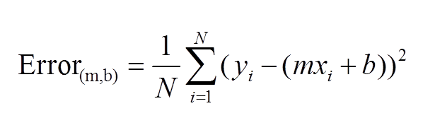
To use the matrix version of the least squares solution
Calculating least squares weights
reading data on dist to return Pandas DataFrame
select data by column
implement column cutoffs

This cell imports the necessary modules and sets a few plotting parameters for display

%matplotlib inline
import numpy as np
import pandas as pd
import matplotlib.pyplot as plt
plt.rcParams['figure.figsize'] = (20.0, 10.0)

Read in the data

Shift + Enter, or press the play button above ^^^

tr_path =r'C:\Users\hp\Downloads\train.csv'
test_path =r'C:\Users\hp\Downloads\test.csv'
data = pd.read_csv(tr_path)

The .head() function shows the first few lines of data for perspecitve

data.head()

-------------------------------------------------------------------------------------------------------

We can plot the data as follows

Price v. living area

with matplotlib

Y = data['SalePrice']
X = data['GrLivArea']

plt.scatter(X, Y, marker = "x")

Annotations

plt.title("Sales Price vs. Living Area (excl. basement)")
plt.xlabel("GrLivArea")
plt.ylabel("SalePrice");

price v. year

Using Pandas

data.plot('YearBuilt', 'SalePrice', kind = 'scatter', marker = 'x');

-------------------------------------------------------------------------------------------------------

Build a function that takes as input a matrix

return the inverse of that matrix

assign function to "inverse_of_matrix"

def inverse_of_matrix(mat):
matrix_inverse = np.linalg.inv(mat)
return matrix_inverse

Testing function:

print("test:\n",inverse_of_matrix([[1,2],[3,4]]), "\n")
print("From Data:\n", inverse_of_matrix(data.iloc[:2,:2]))

In order to create any model it is necessary to read in data

Build a function called "read_to_df" that takes the file_path of a .csv file.

Use a pandas functions appropriate for .csv files to turn that path into a DataFrame

Use pandas function defaults for reading in file

Return that DataFrame

the returned item is of type "DataFrame" and the dimensions should be correct

import pandas as pd
def read_to_df(file_path):
"""Read on-disk data and return a dataframe."""
tr_path =r'C:\Users\hp\Downloads\train.csv'
data = pd.read_csv(tr_path) # making dataframe from the csv file
return data

Testing function:

print(type(data))
print(data[:10])

-------------------------------------------------------------------------------------------------------

Build a function called "select_columns"

As inputs, take a DataFrame and a list of column names.

Return a DataFrame that only has the columns specified in the list of column names

check type of object, dimensions of object, and column names

def select_columns(data_frame, column_names):
tr_path =r'C:\Users\hp\Downloads\train.csv'
data = pd.read_csv(tr_path)
#selected_columns = data.iloc[:,lambda data:data.columns.str.contains('SalePrice|GrLivArea|YearBuilt',case=False)].head()
#fields=['SalePrice','GrLivArea','YearBuilt']
#data2=pd.read_csv(r'C:\Users\hp\Downloads\train.csv', skipinitialspace=True, usecols=fields)
selected_columns = data.loc[:,['SalePrice', 'GrLivArea', 'YearBuilt']]
sub_df = select_columns(data, selected_columns)
return sub_df

#print(data.columns)
#print(data['SalePrice'],data['GrLivArea'],data['YearBuilt'])

-------------------------------------------------------------------------------------------------------

Build a function called "column_cutoff"

As inputs, accept a Pandas Dataframe and a list of tuples.

Tuples in format (column_name, min_value, max_value)

Return a DataFrame which excludes rows where the value in specified column exceeds "max_value"

or is less than "min_value".

### NB: DO NOT remove rows if the column value is equal to the min/max value

def column_cutoff(data_frame, cutoffs):
"""Subset data frame by cutting off limits on column values.

Positional arguments:
data -- pandas DataFrame object
cutoffs -- list of tuples in the format:
(column_name, min_value, max_value)

Example:
data_frame = read_into_data_frame('train.csv')

Remove data points with SalePrice < $50,000

Remove data points with GrLiveAre > 4,000 square feet

cutoffs = [('SalePrice', 50000, 1e10), ('GrLivArea', 0, 4000)]
selected_data = column_cutoff(data_frame, cutoffs)
"""
cutoffs = [('SalePrice', 50000, 1e10), ('GrLivArea', 0, 4000)]
selected_data = column_cutoff(data_frame, cutoffs)

return ''

-------------------------------------------------------------------------------------------------------

Build a function called "least_squares_weights"

take as input two matricies corresponding to the X inputs and y target

assume the matricies are of the correct dimensions

Step 1: ensure that the number of rows of each matrix is greater than or equal to the number

of columns.

### If not, transpose the matricies.

In particular, the y input should end up as a n-by-1 matrix, and the x input as a n-by-p matrix

Step 2: prepend an n-by-1 column of ones to the input_x matrix

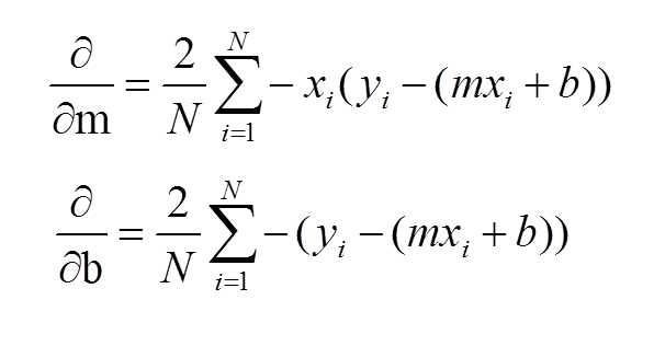
Step 3: Use the above equation to calculate the least squares weights.

NB: .shape, np.matmul, np.linalg.inv, np.ones and np.transpose will be valuable.

If those above functions are used, the weights should be accessable as below:

weights = least_squares_weights(train_x, train_y)

weight1 = weights[0][0]; weight2 = weights[1][0];... weight<n+1> = weights[n][0]

def least_squares_weights(input_x, target_y):

training input

X=np.array([[1710, 1262, 1786,
1717, 2198, 1362,
1694, 2090, 1774,
1077],
[2003, 1976, 2001,
1915, 2000, 1993,
2004, 1973, 1931,
1939]])

column vector form

X=X.T
print(" The shape of the training input matrix:\n", X.shape)

training label

Y=np.array([[208500, 181500, 223500,
140000, 250000, 143000,
307000, 200000, 129900,
118000]])

column vector form

Y=Y.T
print(" The shape of the training label matrix:\n", Y.shape)
print("There are {} numbers of samples".format(X.shape[0]))
print("There are {} numbers of features".format(X.shape[1]))

#Fetching the input data to include bias
X_tilde=np.c_[np.ones([num_samples,1]),X]
print("X_tilde is:\n", X_tilde)

transpose of the input data

X_tilde_T=X_tilde.T

solving the normal equation (using pseudo-inverse instead of inverse because you cannot guarantee

#that the inverse actually exists)

param_tilde= np.linalg.pinv(X_tilde_T.dot(X_tilde)).dot(X_tilde_T).dot(Y)

the optimised parameter (bias + weights)

print("The optimised parameter:\n", param_tilde)

-------------------------------------------------------------------------------------------------------

df = read_to_df(tr_path)
df_sub = select_columns(df, ['SalePrice', 'GrLivArea', 'YearBuilt'])

cutoffs = [('SalePrice', 50000, 1e10), ('GrLivArea', 0, 4000)]
df_sub_cutoff = column_cutoff(df_sub, cutoffs)

X = df_sub_cutoff['GrLivArea'].values
Y = df_sub_cutoff['SalePrice'].values

reshaping for input into function

training_y = np.array([Y])
training_x = np.array([X])

weights = least_squares_weights(training_x, training_y)
print(weights)

-------------------------------------------------------------------------------------------------------

max_X = np.max(X) + 500
min_X = np.min(X) - 500

Choose points evenly spaced between min_x in max_x

reg_x = np.linspace(min_X, max_X, 1000)

Use the equation for our line to calculate y values

reg_y = weights[0][0] + weights[1][0] * reg_x

plt.plot(reg_x, reg_y, color='#58b970', label='Regression Line')
plt.scatter(X, Y, c='k', label='Data')

plt.xlabel('GrLivArea')
plt.ylabel('SalePrice')
plt.legend()
plt.show()

-------------------------------------------------------------------------------------------------------

Calculating RMSE

rmse = 0

b0 = weights[0][0]
b1 = weights[1][0]

for i in range(len(Y)):
y_pred = b0 + b1 * X[i]
rmse += (Y[i] - y_pred) ** 2
rmse = np.sqrt(rmse/len(Y))
print(rmse)

-------------------------------------------------------------------------------------------------------

Calculating 𝑅2

ss_t = 0
ss_r = 0

mean_y = np.mean(Y)

for i in range(len(Y)):
y_pred = b0 + b1 * X[i]
ss_t += (Y[i] - mean_y) ** 2
ss_r += (Y[i] - y_pred) ** 2
r2 = 1 - (ss_r/ss_t)

print(r2)

-------------------------------------------------------------------------------------------------------

sklearn implementation

from sklearn.linear_model import LinearRegression

lr = LinearRegression()

sklearn requires a 2-dimensional X and 1 dimensional y. The below yeilds shapes of:

skl_X = (n,1); skl_Y = (n,)

skl_X = df_sub_cutoff[['GrLivArea']]
skl_Y = df_sub_cutoff['SalePrice']

lr.fit(skl_X,skl_Y)
print("Intercept:", lr.intercept_)
print("Coefficient:", lr.coef_)

Overflow when learning rate is too small

After changing the learning rate from 0.0001 to 0.001 the demo program overflows. Any insights about what is going on? J

After 1000 iterations b = nan, m = nan, error = nan

While running the code getting following error:-

Starting gradient descent at b = 0, m = 0, error = nan
Running...
After 1000 iterations b = nan, m = nan, error = nan
plottting..

Code:-

import numpy as np
import pandas as pd
import math
import matplotlib
import matplotlib.pyplot as plt
from sklearn import datasets, linear_model
from pandas import DataFrame, Series
from sklearn.metrics import mean_squared_error

data = pd.read_csv("http://archive.ics.uci.edu/ml/machine-learning-databases/auto-mpg/auto-mpg.data-original",
delim_whitespace = True, header=None,
names = ['mpg', 'cylinders', 'displacement', 'horsepower', 'weight', 'acceleration',
'model', 'origin', 'car_name'])

#The optimal values of m and b can be actually calculated with way less effort than doing a linear regression.
#this is just to demonstrate gradient descent

from numpy import *

y = mx + b

m is slope, b is y-intercept

def compute_error_for_line_given_points(b, m, points):
totalError = 0
for i in range(0, len(points)):
x = points[i, 0]
y = points[i, 1]
totalError += (y - (m * x + b)) ** 2
return totalError / float(len(points))

def step_gradient(b_current, m_current, points, learningRate):
b_gradient = 0
m_gradient = 0
N = float(len(points))
for i in range(0, len(points)):
x = points[i, 0]
y = points[i, 1]
b_gradient += -(2/N) * (y - ((m_current * x) + b_current))
m_gradient += -(2/N) * x * (y - ((m_current * x) + b_current))
new_b = b_current - (learningRate * b_gradient)
new_m = m_current - (learningRate * m_gradient)
return [new_b, new_m]

def gradient_descent_runner(points, starting_b, starting_m, learning_rate, num_iterations):
b = starting_b
m = starting_m
for i in range(num_iterations):
b, m = step_gradient(b, m, array(points), learning_rate)
return [b, m]

def plot_dp():

Input_file = np.genfromtxt('auto-mpg1.csv', delimiter=',', skip_header=1)
Num = np.shape(Input_file)[0]
X = np.hstack((np.ones(Num).reshape(Num, 1), Input_file[:, 4].reshape(Num, 1)))
Y = Input_file[:, 0]

X[:, 1] = (X[:, 1]-np.mean(X[:, 1]))/np.std(X[:, 1])

wght = np.array([0, 0])

max_iter = 1000
eta = 1E-4
for t in range(0, max_iter):
    grad_t = np.array([0., 0.])
    for i in range(0, Num):
        x_i = X[i, :]
        y_i = Y[i]
      
        h = np.dot(wght, x_i)-y_i
        grad_t += 2*x_i*h
 
    wght = wght - eta*grad_t


tt = np.linspace(np.min(X[:, 1]), np.max(X[:, 1]), 10)
bf_line = wght[0]+wght[1]*tt

plt.plot(X[:, 1], Y, 'kx', tt, bf_line, 'r-')
plt.xlabel('displacement (Normalized)')
plt.ylabel('MPG')
plt.title('Linear Regression')
plt.show()

def run():
points = genfromtxt("data.csv", delimiter=",")
learning_rate = 0.0001
initial_b = 0 # initial y-intercept guess
initial_m = 0 # initial slope guess
num_iterations = 1000
print "Starting gradient descent at b = {0}, m = {1}, error = {2}".format(initial_b, initial_m, compute_error_for_line_given_points(initial_b, initial_m, points))
print "Running..."
[b, m] = gradient_descent_runner(points, initial_b, initial_m, learning_rate, num_iterations)
print "After {0} iterations b = {1}, m = {2}, error = {3}".format(num_iterations, b, m, compute_error_for_line_given_points(b, m, points))

print('plottting..')
plot_dp()

if name == 'main':
run()

Function compute_error_for_line_given_points not required.

The first function does not serve any purpose and makes the code lengthy. And for beginners like me, confuses people. The program runs fine without any such function as the work of that is done in the step_gradient function itself.