luggs123/simplemultilayerperceptron

Easy to understand demo/guide of a type of neural network, an MLP.

Simple Multilayer Perceptron Example by Farza

Simple example to understand how the most basic neural network is actually working. To run it:

git clone https://github.com/farzaa/SimpleMultilayerPerceptron.git
cd SimpleMultilayerPerceptron
pip install numpy
python simple_mlp.py

Make sure you have Python 2 installed, since this does not run in Python 3. As for prior knowledge, know how Python works and the basics of calculus/matrix algebra.

I don't go over how numpy works in this tutorial but just imagine it as a super cool/easy library to work with matrixes and many other things. Every numpy method call will have an np come before it. If you don't get what it's doing, refer to this easy doc: http://cs231n.github.io/python-numpy-tutorial/

Here is our input/ output:

Input	Output
0 0 1	0
1 1 1	1
1 0 1	1
0 1 1	0

Really understand this input/output, whats going on? Notice how there is a unique output for every single input. Think of this as a linear relationship where the function representing our input/output is linear.

We are going to build a simple neural network known as an multi layer perceptron to learn how to solve this function. This is a really good exercise that helped me a ton to understand lots of terminology and core concepts related to neural networks and deep learning.

Let's look at the train method which is where all the magic happens.

def train(inputs, keys, weights):
  for iter in xrange(20000):
	  prediction = applySigmoid(np.dot(inputs, weights))
	  error = keys - prediction
	  change_in_error = error * applySigmoid(prediction,True)
	  weights += np.dot(inputs.T ,change_in_error)

We'll look at the number of iterations iter later.

The first thing we do is calculate our prediction np.dot(inputs, weights) which is basically forward propagation where we dot the inputs by the weights at that current iteration. What exactly are the weights doing?

We want the weights to account for the relationship between the input and the output. For example, imagine I was training a neural network that helped me figure out what foods I liked best. I'd train the network by giving it a bunch of foods I liked (ex. ice cream, pizza, orange chicken) and didn't like (peas, carrots, etc). How does the network actually "learn" what foods I like and don't like? By adjusting the weights and understanding the RELATIONSHIP between the attributes (ex. ingredients, color, etc) of each food and whether or not I like them.

Let's say a specific (single) neuron in my network focused on if I would like a food based on how sweet that food was. I train this by inputting all the stuff I eat. The weights are adjusted so that food that is more sweet has an output of "LIKE" and food that is not sweet has an output of "DISLIKE". The weights are adjusted every single iteration of training by some amount, slowly it is this weight matrix that gets "smarter" and has the ability to make decisions on its own because it understands the function between food, sweetness, and LIKE or DISLIKE

Side note: This isn't completely right because I like pizza, but pizza isn't sweet! Though, remember this is just a single neuron in our network. Imagine our network outputs a final "LIKE" or "DISLIKE" based on all the outputs of all the different nodes (ex. a node for savory food, a node for green colored food, a node for oily food).

Let's get more technical. Back to the code.

prediction = applySigmoid(np.dot(inputs, weights))

At iteration 0, our weights are initialized to some random values (more on this later) and haven't been trained yet which means are prediction will most likely be very wrong. But lets see it for ourselves.

The first iteration iter = 0. Our inputs are dotted with the weights, remember these are initially random! A 4x3 matrix dotted with a 3x1 matrix is proper input and will give us a 4x1 matrix which is exactly right since the size of keys is 4x1 as well.

[[0 0 1]            [[ 0.18599833]
 [1 1 1]    dot      [ 0.51668113] 
 [1 0 1]             [-0.80185633]]
 [0 1 1]]

Keep in mind that the values you see here will be different from the ones you get yourself, since our random weights are initialized separately. Your results won't be the same, but they will be similar. This 4x1 matrix result is our prediction, and we get:

[[0.2689864]
[0.3262757]
[0.23762817]
[0.36375058]]

Remember our keys are:

[[0]
[1]
[1]
[0]]

Our prediction is WAY off. But that is to be expected at iteration 0 because our system hasn't been trained at all. It just picked random weights and hoped for the best. Once we find this dot product we do applySigmoid() on it. This is the activation function and this specific activation function introduces nonlinearity into our model. Let's break this down.

An activation function (from Wikipedia) "defines the output of that node given an input or set of inputs". When we do np.dot(inputs, weights), this gives us a combination based on the LINEAR relationship of the two matrixes. Let's see why we don't necessarily want linearity in our models.

Look at this situation below. Imagine the black dots are junk foods I love/hate sometimes and white dots are vegetables I love/hate sometimes and this is the output of a network that decided how much I liked these two types of foods. How would you draw a line separating these two classes from each other?

Try as much as you can and you'll find that there is no solution by simply drawing a line. This means the issue of deciding what foods I like is a NONLINEAR problem.

This output above actually comes from the XOR truth table, and the way we separate the two classes is via a nonlinear solution.

Imagine if you had a MASSIVE neural network with many layers and nodes that decided my favorite foods. Now imagine this net didn't utilize a nonlinear activation function like Sigmoid or something else. This means our big, complex neural network is only as good as a single layer perceptron! WTF WHY?? This is because summing up a bunch of linear functions is going to just give us another linear model and we get the same problem as the XOR issue above. We need nonlinearity in the model to avoid this issue of our big, fancy neural net boiling down to a single layer perceptron.

This is where the Sigmoid function comes in.

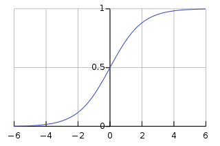
It is a differentiable (important later) nonlinear function and it will squash any number (from - infinity to infinity) to a number between 0 and 1.

So here the line once again

prediction = applySigmoid(np.dot(inputs, weights))

And our output at iteration 0 is going to be. Notice how every number has been "squashed" between 0 and 1.

[[ 0.56684405 ]
 [ 0.58085292 ]
 [ 0.559129067]
 [ 0.589948040]]

In summary, we are using forward propagation using our weights and inputs to predict the right answer and we are using the activation function to introduce nonlinearity.

On to the next line

error = keys - prediction

Here we are, at the simplest level, we're calculating loss by subtracting the right answers from our predictions and saving that difference. This essentially says "By how much was I off from the right answer?". We use this to adjust our weights later. Let's talk about this a little more before getting to the next part.

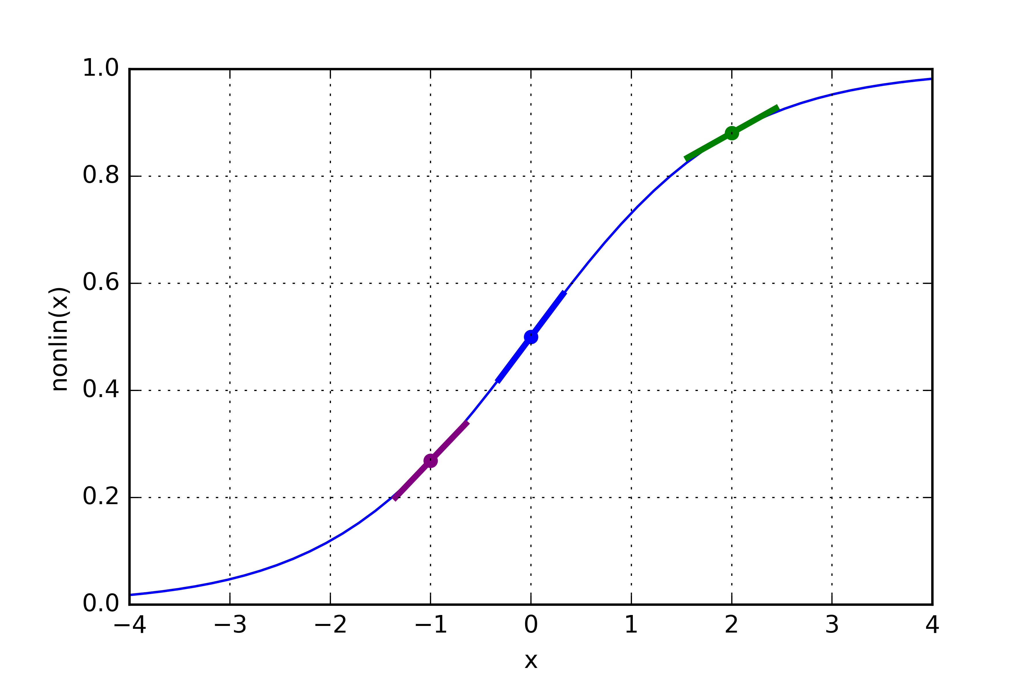
Above is the Sigmoid function again, but this time the slopes are highlighted. You'll notice that the slopes near the top and bottom are relatively shallow but the slopes near the center are much steeper. We can calculate these exact slopes by finding the derivative of the Sigmoid function and plugging in a value for x. These slopes essentially tell us how right or wrong we were. Something to keep in mind is that the neural network will never be exactly right, but we can get pretty damn close.

If we were WRONG, than the slope will be like the slope in the center and we'll change our weights by some factor of this slope.

If we CLOSE TO BEING CORRECT, than the slope will be shallow and we'll STILL change our weights but it will change by some much smaller factor since our slope is much smaller.

This makes sense because we want to change our weights by a larger amount if we were wrong and a smaller amount if we're close to right. This method is known generally as back propagation and it's the soul of machine learning.

Let's think of backpropagation a different way just to make sure I properly sell this idea to you. Imagine you're playing a video game like, League of Legends or Call of Duty, but you are absolutely terrible at it and don't understand why you aren't improving. Your keep spawning and running straight to the enemy base and getting killed like our friend in the GIF below. What's the issue here?

You aren't learning from your mistakes. Lets try this, everytime you die, think about why you died and try not to make that same mistake again. This is how backpropagation is working. You're learning based on past mistakes and adjusting yourself accordingly. You might not get good in a couple days, but after a couple of weeks you might look like this guy:

The back propagation method I'm going to use below (and the one I explained above with the slopes) is called the Delta Rule which is also called The Error Weighted Derivative and this is a VERY simple way to help you understand backpropagation. More complex networks use more complex backpropagation methods, but this is a simple perceptron with a single layer so we can keep it simple to just make sure everything is easy and understandable.

Back to the code. Here's the line we are on:

change_in_error = error * applySigmoid(prediction,True)

I pass True to the applySigmoid function to tell it to do its calculations with the derivative rather than the plain Sigmoid function. Here's the function for reference:

def applySigmoid(x, giveMeTheDerivative = False):
	if(giveMeTheDerivative == True):
		return applySigmoid(x) * (1 - applySigmoid(x))
	return 1 / (1 + np.exp(-x))

So when we do error * applySigmoid(prediction,True) we are adjusting our error matrix by a factor equivalent to the slope of our predictions. This way, if we had a small error and a small slope for that prediction, we are going to change our weights slightly. But if we have a big error, our slope will be much larger as well so we are going to change our weights by a larger factor.

And finally, the last line:

weights += np.dot(inputs.T ,change_in_error)

Why do we do dot the transpose of the inputs with the change in error? The transpose is done so that the math works out. The actual dot happens so that we adjust our weights with respect to our inputs.

Answer to two questions I had that were very important to my understanding of this code:

1. You may be asking yourself, why do we even need this concept of a slope? Why can't we just adjust our weight matrix based on the error? This comes down to that concept of nonlinearity. If we only use the error matrix, where error = keys - prediction, to adjust the matrix than we're just adjusting the weights by some linear function and our neural network is just as good a single layer perceptron.

2. Why can't we just adjust our weight matrix based on the slopes? It is very important to understand this concept. You may notice that we did not adjust our weight matrix at all until the very end. We first adjust our error matrix by multiplying by our slopes, and THAN we change our weight matrix. But why is this, why not just multiply the SLOPES by the elements in our WEIGHT matrix? Wouldn't this also adjust our weight matrix based on how wrong or right we were? NOPE. All our slope is telling us is how confident the prediction was. We need to adjust our error BASED on how confident we were. You need to know where you were wrong or right and adjust the weights accordingly based on this.

3. I mentioned above that having a big neural network with a nonlinear activation function is just as good as a neural network that is one layer deep. Recall, we used a nonlinear activation function here. Does that mean this specific neural network in nonlinear? NOPE. This neural network has only a single layer right now, so it doesn't matter that we have this fancy activation function because the network itself can only understand one to one relationships.

Point #3 brings me to my next example and probably the most important of this guide when it comes to deep learning. Let's look at the input I gave you again.

Input	Output
0 0 1	0
1 1 1	1
1 0 1	1
0 1 1	0

Remember, how every input/output has a linear relationship in this specfic table? Lets change our input/output to look like the XOR truth table I mentioned above not to long ago.

Input	Output
0 0 1	0
1 0 1	1
0 1 1	1
1 1 1	0

Lets run this input/output through our simple_mlp.py program. Just change the values of input and keys. Lets run our network with this new input, train it, and see if it gets the right prediction.

Here is the prediction after 10 K iterations.

[[ 0.5]
 [ 0.5]
 [ 0.5]
 [ 0.5]]

RATS! Our neural network is broken! Well, kinda. It's just not fit for the task at hand. Lets explore why we get this very incorrect output. Take a look at the input again.

Two 0s leads to a 0. Okay cool. one 1 and one 0 leads to a 1. Okay cool. One 0 and one 1 leads to a 1. Wait, hmmmm. The same inputs in a different order leads to the same result? Yes. XOR only evaluates to true if either the inputs are true.

What does this mean? Our input isn't simply one to one (linear). The relationship between our inputs leads to our output. This is a nonlinear problem and our current neural network is unable to solve it because our MLP only has one hidden layer. It needs another hidden layer to better understand the relationship between the inputs and to better understand how the output is achieved.

Still don't get it? Lets think about it mathematically for a second.

f(output layer one) = InputsLayerOne * WeightsLayerOne
f(output layer two) = f(output layer one) * WeightsLayerTwo

The input to our second layer is a function of the previous layer. In a deep neural network, this behavior is what allows us to capture much more profound and complex attributes like birds in an image or number of faces in a video.

Okay, so how do we fix it? Like I said above, add another hidden layer. You can see how this is done in fancy_mlp.py. As long as you understand the simpler example, the more complex example shouldn't be an issue.

Two things I didn't cover and will write up later:

• Weight initialization
• Weight matrix shape