"SATELLITE" Documentation

Dr. Stavros Akras

Institute for Astronomy, Astrophysics, Space Applications and Remote Sensing,

National Observatory of Athens

2021

Introduction

The Spectroscopic Analysis Tool for intEgraL fieLd unIt daTacubEs (Satellite) is a newly developed code for the spectroscopic characterization of extended photo-ionised nebulae such as planetary nebulae, H II regions or galaxies in the optical regime observed with any integral field unit (IFU). SATELLITE has been written in python and was developed to be an automatic and user-friendly code. The user does not need any programming or coding knowledge.

The capabilities and performance of the satellite code (v1.0) were presented using the IFU data of the Abell~14 PN obtained with VIMOS@ESO. Satellite v1.3 has been applied to three more PNe: Hen 2-108 (VIMOS) (Miranda Marques et al. 2021, submitted), NGC 7009 (MUSE), and NGC 6778 (MUSE) (Akras et al. 2021, submitted).

Satellite carries out a spectroscopic analysis of extended ionized nebulae through 1D and 2D approach on a list of 35 emission line (the brightest and more frequently detected in ionized nebulae) via a number of pseudo-slits that simulate slit spectrometry and 2D emission line imaging. The analysis is performed in four different modules:

(I) rotation analysis,
(II) radial analysis,
(III) specific slits analysis and
(IV) 2D analysis

For each module, satellite computes all the typically used nebular parameters and their uncertainties using as input information the available emission lines maps. For all four modules, the uncertainties of the line intensities as well as those of the nebular parameters are computed following a Monte Carlo approach considering a number of spectra.

extinction coefficient (c(Hbeta)),
electron temperatures and densities for different diagnostic lines,
ionic and elemental abundances, abundances ratio relative to oxygen and the ionization correction factors,
emission line ratios from a pre-defined list

The input parameters necessary to run the code are provided by the user in four ASCII files:

input.txt
numerical_input.txt
output.txt (the requested outputs from the code!)
diagnostic_diagrams_input.txt
plots_parameters_input.txt

and they are:

emission line and error maps (or additional error as percentage of its pixel flux. )
the pixel scale of the IFU
the interstellar extinction law
number of replicate spectra
the width, length, position angle (PA) and coordinates of the pseudo-slits for the 1D analysis
the coordinates of the central star or the centre of the nebula
atomic data
Te and Ne from different diagnostic lines for the proper calculation of the ionic abundances
the line ratios that the code will compute
the emission line diagnostic diagrams that the code will construct
the module or modules that the code will execute

The philosophy behind the development of the satellite code is, besides the unique 2D imaging spectroscopy that IFU technology provides, to carry out a detailed 1D spectroscopic analysis through a number of pseudo-slits that simulate slit spectrometry and emission line imaging in order to properly compare the results presented in previous studies. The outputs from each of satellite’s modules are saved in five different folders:

output_angles_plots (\leftarrow) rotation analysis module
output_Diagnostic_Diagrams (\leftarrow) 2D analysis module
output_images (\leftarrow) 2D analysis module ( & slit position testing)
output_plots (\leftarrow) 2D analysis module
output_radial_plots(\leftarrow) radial analysis module

The description of each module as well as the input parameters and outcomes are described in more details in the following sections using as a representative example the analysis of the planetary nebulae NGC 7009 and its MUSE data from the Science Verification phase .

Set up and Run the SATELLITE Code

Satellite has been successfully run/tested in Fedora 23 operation systems and Python version 3.9.7. To use the satellite code, it is also necessary to install a number of libraries such as matplotlib, numpy, scipy, astropy, and seaborn libraries.

The version of the libraries was: matplotlib v2.2.5, numpy v1.11.1 and scipy v0.18.0, astropy v2.0.12, and seaborn v0.9.1. satellite also make use of the PyNeb package version 1.1.15 .

The installation of a library can be done via pip and the command: pip install library.

To get the version of the installed libraries add the following lines in a python script and run it.

import matplotlib import numpy import seaborn import astropy import scipy)

print(matplotlib.version) print(numpy.version) print(seaborn.version) print(astropy.version) print(scipy.version)

For the atomic data from the Chianti database, it is necessary to download the data from the website https://www.chiantidatabase.org/.

GitHub repository

Download {\sc satellite} from GitHub (https://github.com/StavrosAkras/SATELLITE) command: "** git clone https://github.com/StavrosAkras/SATELLITE.git **" A new folder will be created namely SATELLITE with all the necessary files.
run setup.py in the satellite folder command: "python setup.py install" Setup.py also installs all the necessary python packages need to use satellite included Pyneb
run the code command: "** ./satellite $>$ outputLog.txt **"

A number of general comments provided from the different modules of the code are written in the outputLog.txt ASCII file.

READ INPUT DATA

The number of input data that the user has to provide the code.

read_input_script

In the current version of satellite, there is a pre-defined list of 35 emission lines from which the user can select the emission line that will be used by the code for the analysis. The list contains the most commonly detected and relatively bright emission line in ionized nebula such as the H and He recombination lines (recombination lines from O or N will be implemented to future versions) and collisionaly excited lines from O+, O++, N+, N++ ,S+, S++, etc. (see Figure 1.

Fig. 1. Example of the input.txt file from which the user can select the emission line that will be used for 1D spectroscopic analysis or radial analysis.

The user can access the list from the input.txt file and just add "yes" or "no" in the second column for both flux and error maps. The first column in the input.txt lists the name of the emission lines. The input "FIT files" of the emission line map must have the same name. Moreover, all the input "FIT files" (maps) must be located in the image_data folder. Hint: In case error maps are not available, the user can create some fake error maps by multiplying the flux maps by e.g. 0.1 to replicate an uncertainty of 10 percent for each emission line. The option of an extra error is also possible. In the forth column, the user can add an extra error for each line as a percentage of the flux (e.g. 1% of the total flux of [O III]5007A line). The even rows for each line (error lines) can take two numerical values "0" and "any integer". (i) "O" means that the final error for each pixel and each emission line is equal to the percentage of the flux, and (ii) "any number" means that the final error for each pixel and each emission line is equal to the error from the error map + the percentage of the flux.

The third column in the input.txt deals with the radial_analysis module and the user adds, "radial_yes " or " radial_no ", for the lines(with their error maps) are available and will be used for this module. Note: The Halpha and Hbeta lines must always be selected for the determination of the interstellar extinction coefficient and corrected line intensities.

The read_input_script reads the flux and error maps of each line defined in the input.txt file pixel-by-pixel and save the values in 2D arrays.

For the example of NGC 7009, the selected emission lines are presented in Figure 1.

read_input_lines_parameters_script

Besides the selection of the emission line and error maps, there is also a list of numerical parameters that the code needs to run properly and they are provided by the user in different files. All these parameters are read by the code via the read_input_lines_parameters_script. Below, the most important parameters are listed together with the ascii files:

the pixel scale of the IFU in arcsec (x10(^{2})) -> numerical_input.txt
the interstellar extinction law (Rx10(^{1})) -> numerical_input.txt
atomic data -> numerical_input.txt
the width, length, position angle (PA) and coordinates of the pseudo-slits for the 1D analysis in the rotation_analysis, radial_analysis, and specific_slits_analysis modules -> numerical_input.txt
the coordinates of the central star or the centre of the nebula -> numerical_input.txt file
number of replicate spectra for the determination of the uncertainties -> numerical_input.txt file
the minimum radius from which the maximum line flux will be determined and the profiles will be normalized to 1. -> numerical_input.txt file
the number of column and row pixels that have to be added to the raw maps in order to put the centre of the nebula at the center of the map -> numerical_input.txt
the module or modules that the code will execute -> outputs.txt file
the emission line ratios that the code will compute based on the available line maps -> outputs.txt
the physical parameters (c, Te, Ne that the code will compute based on the available line maps -> outputs.txt
the Te and Ne from specific diagnostic lines that will be used to compute ionic abundances -> outputs.txt
the elemental abundances and ICFs that the code will compute based on the available line maps -> outputs.txt
the diagnostic diagrams that the code will construct -> diagnostic_diagrams_input.txt
the xmin/xmax and ymin/ymax for the diagnostic diagrams -> diagnostic_diagrams_input.txt
if the user wants to over-plot the selection criteria from Kewley2001 and Kauffmann2003 -> diagnostic_diagrams_input.txt
ymin/ymax for the scatter plots -> plots_parameters_input.txt file

Reorder line flux and error maps

The first task the user must perform before run satellite is to compute the number of columns and rows of pixels that need to be added to the raw line flux and error maps in order to put the central star or centre of the nebula at the centre of the new map. This task is very important in order to properly rotate the maps and measure the line fluxes in each pseudo-slit. Note: The final maps have to have the same number of columns and rows!

Figure 2 presents a cartoon that illustrates the numbers of rows of pixels need to be added to the top and bottom of the raw map as well as the columns of pixels to the left and right parts of the raw maps. The value these extra pixels have is zero and they do not have any impact on the spectroscopic analysis. The extra row and columns added in the flux and error maps are provided by the user in the numerical_input.txt file.

CM (15,15) is the centre of the raw map and CS (19,12) is the central star of an ellipsoidal planetary nebula (orange colour). The offset between the CS and CM is 4 pixels in row and 3 pixels is column. It is necessary to move the CS to the left and up by adding some extra columns and rows. So, 8 columns are added to the right side and the CS is now in the middle (19,19) and 6 rows at the bottom so the CS is now at the position (18,18). But the map still does not have the same number of columns and rows (38,36). For this reason, we have to add 1 extra row to the top and 1 extra to the bottom. Finally, the CS is the centre of the new map at position (19,19). These numbers are added in the numerical_input.txt file as it is show below:

add_pixels_above=1
add_pixels_below=7
add_pixels_left=0
add_pixels_right=8
total_num_pixels_verti=30
total_num_pixels_horiz=38

As for NGC 7009, the number of rows to the top and bottom of the raw maps are 35 and 35, respectively, and the extra columns to the left and right side are 4 and 6, respectively.

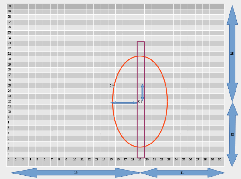
Fig.2 Illustrative example of a line flux map and the rows/columns that have to be added in order to coincide the CS with the CM of the new map.

Extinction Coefficient

Satellite determines the extinction coefficient (c(Hbeta)) using the PyNeb package (see: https://github.com/Morisset/PyNeb_devel/blob/master/docs/Notebooks/PyNeb_manual_5.ipynb) and constructs the 2D map and its error map. All the extinction law available in the the PyNeb can be selected (’No correction’, ’CCM89’, ’CCM89_Bal07’, ’CCM89_oD94’, ’S79_H83_CCM89’, ’K76’, ’SM79_Gal’, ’G03_LMC’, ’MCC99_FM90_LMC’, ’F99’, ’F88_F99_LMC’]). The R parameter is also given by the user (e.g. R=3.1) in the numerical_input.txt file as an integer number (R*10=031). The save_FITSimages_script saves the 2D arrays as FITS image.

The code does not take into account all the pixels in the pseudo-slits or estimates the extinction coefficient for all the pixels BUT only for those that satisfy the following criteria:

F((Ha)) > 0,
F((Hb)) > 0
F((Ha)) > F((Hb))*2.86
otherwise a value "zero" is applied.

There is also an option to find the outliers and exclude them from the calculation of the mean/median values. The outliers are defined as those pixels with values that do not satisfy the criteria: value(>)per25-1.5*iqr and value(<) per75+1.5*iqr), where per25 and per75 are the 25% and 75% percentiles, respectively, and iqr = per75 - per25 the inter-quartile-range. These calculations are made in the calculations_excluding_outliers_script. In the current version, the outliers are not excluded from the physical parameters that the code computes.

Atomic Data

The atomic data can also be changed by the user. All the options available in the PyNeb package can be used by adding in the numerical_input.txt the words: IRAF_09_orig, IRAF_09, PYNEB_13_01, PYNEB_14_01, PYNEB_14_02, PYNEB_14_03’, ’PYNEB_16_01, PYNEB_17_01, PYNEB_17_02, PYNEB_18_01, PYNEB_20_01, and PYNEB_21_01. The atomic data from Chianti group can also be used (adding the word ’’Chianti‘‘in the numerical_input.txt) but they have to be downloaded from the website ( http://www.chiantidatabase.org/chianti_download.html.). For more information the user must refer to the website of PyNeb package (https://github.com/Morisset/PyNeb_devel/blob/master/docs/Notebooks/PyNeb_manual_3.ipynb)

SATELLITE’s Modules

The modules that the code executes are defined in the second column ("yes" or "no") of the outputs.txt file. Each module is described below. Note: It is recommended to run the radial_analysis module separately from the other three modules.

rotation_analysis module

The rotation_analysis module deals with the spectroscopic analysis of a number of radial placed pseudo-slits from the centre to outer parts with position angles (PA) between 0 and 360. Figure 3 illustrates as example the position of these pseudo-slits on the [N II] 6584 emission line map of NGC 7009. The minimum and maximum values of the PA, the step in PA , the width and the length of the pseudo-slits are provided by the user in the file numerical_input.txt.

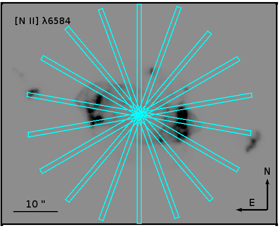
Fig.3 An illustrative image of the radial positioned pseudo-slits with PA from 0 to 360 every 20 degrees overlaid the [N II] 6584 image of NGC 7009.

The code first computes the integrated H(beta) flux and line fluxes in the rotate_line_fluxes_script. Then, line intensities (relative to H(beta) and corrected for the interstellar excitation) as well as all the nebular parameters defined by the user in the output.txt file for all the pseudo-slits are computed by the PyNeb package. This analysis allows to explore the variation of line intensities, line ratios and physical parameters (Te, Ne), chemical abundances as functions of PA.

The outcomes from this module are multiple and are saved in different files:

an ASCII file with the c(H(beta)) and the intensity of each emission line and for each PA -> output_linesintensities_per_angles.txt
an ASCII file with various line ratios defined by the user for each PA -> output_lineratios_per_angles.txt
an ASCII file with Te and Ne defined by the user for each PA -> PyNeb_output_Te_and_Ne_per_angles.txt
an ASCII file with the ionic abundances for each ion defined by the user for each PA -> PyNeb_output_total_abund_ICFs_per_angles.txt
an ASCII file with the elemental abundances and ICFs for each element defined by the user for each PA -> PyNeb_output_ionic_abund_per_angles.txt
plots of c(H(beta)), Te, Ne, ionic, elemental abundances, ICFs and abundances ratios as function of the PA -> output_angles_plots folder

The user can use the ASCII files to carry out any further analysis and/or construct his/her own proper plots.

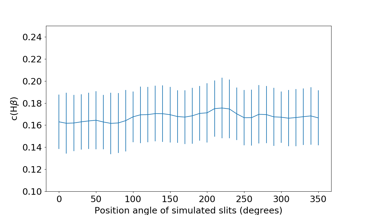
Figure [4] and [5] present the plots of c(H(beta)), Te, Ne, ionic, elemental abundances and ICFs of N as functions of the position angle of the pseudo-slits for the analysis of NGC 7009. Te and Ne are shown in the same plot as in Figures [4] and [5] or in two separate plots.

Fig. 4. Representative plot of c(Hbeta) (upper panel), Te and Ne for two different diagnostic lines (middle/lower panels) as a function of the PA of the pseudo-slits.

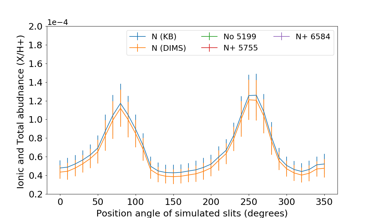
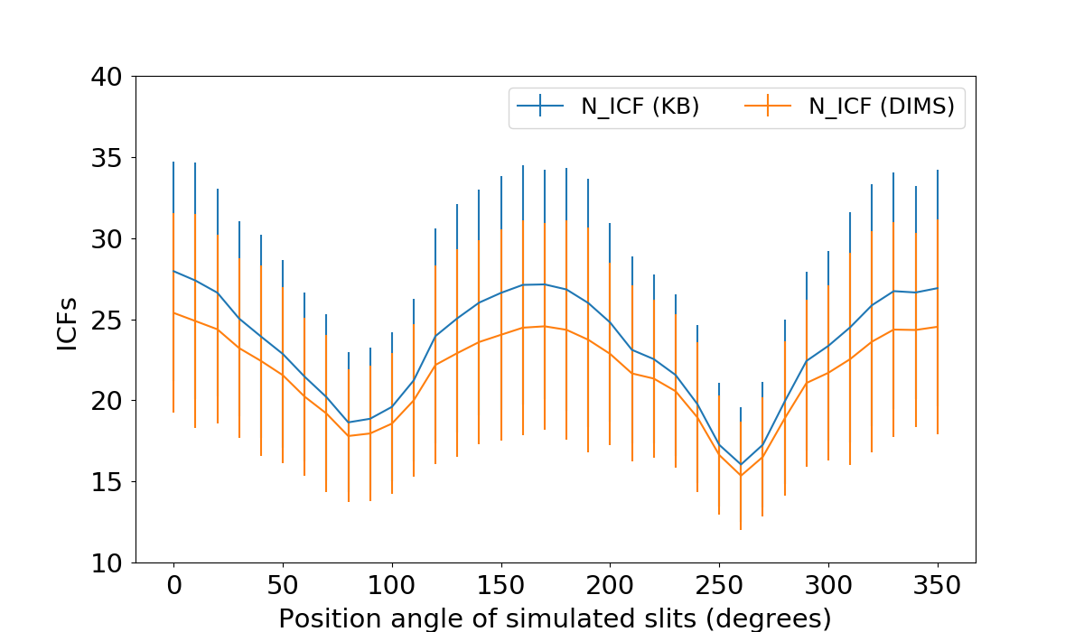
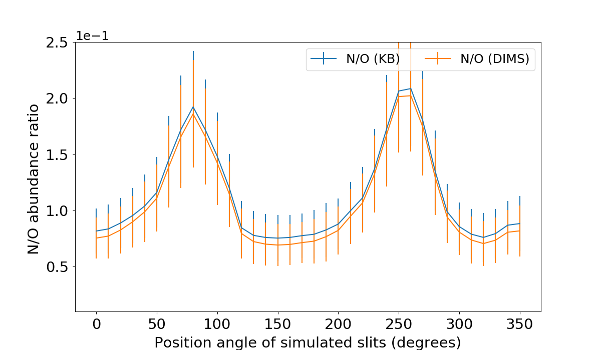
Fig. 5. Representative plot of the ionic/total abundance of N (upper panel), the ICF(N) (middle panel) and the N/O ratio as functions of the pseudo-slits' PA.

slit_line_flux_script

This script calculates the flux for each emission line along a pseudo-slit with a specific position angle, width and length given by the user in the numerical_input.txt file. Note1: The width should always be an integer number. The pseudo-slit starts from the centre of the image or of the nebula, and it covers only one half of the nebula. The code sums up the values of all the pixels within the area defined by the width and length of the pseudo-slit, except those pixels which have F((Ha))(<)0, F(Hb)<0 and/or F(Ha)<F(Hb)*2.86 (negative or unrealistic c(Hb)).

For the calculations, the script first rotates the entire image/table by a given angle, then calculates the new size (x,y) of the rotated imaged as well as the center of the new image. The pseudo-slit is always oriented along the up-down direction of the image. The script computes the total flux for each emission line and the total number of pixels.

Note2: It is necessary the image be large enough to be sure that after the rotation, the entire nebula or galaxy remains inside the image. Sometimes an elongated nebula (or even a galaxy) is observed in a specific PA, so the entire nebula fits the field of view of the instrument (rotation angle=0 in the satellite code corresponds to observed PA=0).
Note3: The orientation of the maps/images should always be north up and east to the left. Otherwise the user has to take into account the offset between the sky (North) and image orientation.

In case, the slit width and length are equal to the number of the pixels in the raw map (parameter total_num_pixels_horiz in the numerical_input.txt file), the code calculates the integrated fluxes of the entire nebula for all the position angles. This specific task was used to verify if the rotation of the images affects the integrated line fluxes.

If the slit width and length are larger than the maximum number the software return the following message: "Sorry, your slit width or/and length are larger than the true size of the image".

TeNe_angles_script, ionicabundances_angles_script and element_abundances_ICFs_angles_script

Te, Ne, ionic/elemental abundances, ICFs and abundance ratios are also computed for each pseudo-slit. Various diagnostic lines can be used for Te/Ne. The user can also choose which T e/Ne combination will be applied for the abundances of each ion (see Figure 6)). All these parameters are defined by the user in the outputs.txt file. Te and Ne parameters are computed in the TeNe_angles_script, while the ionic,elemental abundances and ICFs are computed in the ionicabundances_angles_script and element_abundances_ICFs_angles_script. All the scripts make use of the PyNeb package.

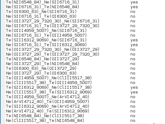
Fig. 5. An example of the outputs.txt file for NGC 7009 and the parameters that the user has to define for the calculations of Te, Ne, ionic/elemental abundances, ICFs and abundance ratios.

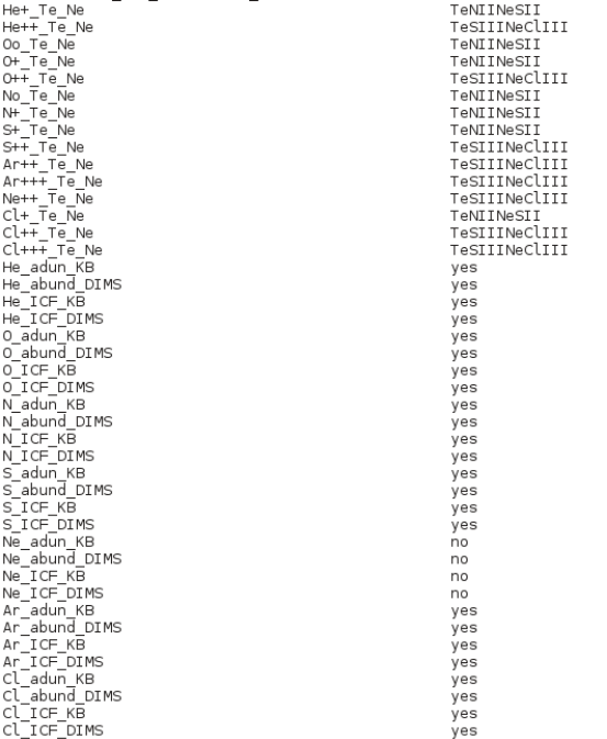
Fig. 6. An example of the outputs.txt file for NGC 7009 and the parameters that the user has to define for the calculations of Te, Ne, ionic/elemental abundances, ICFs and abundance ratios.

specific_slit_analysis module

In this module, the user can define 10 pseudo-slits for a spectroscopic analysis of specific regions/structures in PN (e.g. knots, blobs, inset or outer regions) or in any extended nebula. All the input information from the 10 specific pseudo-slits are given by the user in the numerical_input.txt file:

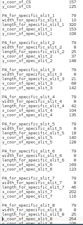
Fig. 7. An example of the numerical_input.txt file for NGC 7009 and the parameters that the user has to define for the 10 pseudo-slits in the specific_slit_analysis module.

PA_for_specific_slit_n (in angle)
width_for_specific_slit_n (in pixels)
length_for_specific_slit_n (in pixels)
x_coor_of_spec_slit_n (in pixels)
y_coor_of_spec_slit_n (in pixels)

where n is the number of the pseudo-slit from 1 to 10 (see Figure 7). The x_coor_of_spec_slit_n, and y_coor_of_spec_slit_n parameters refer to the centre of each slit.

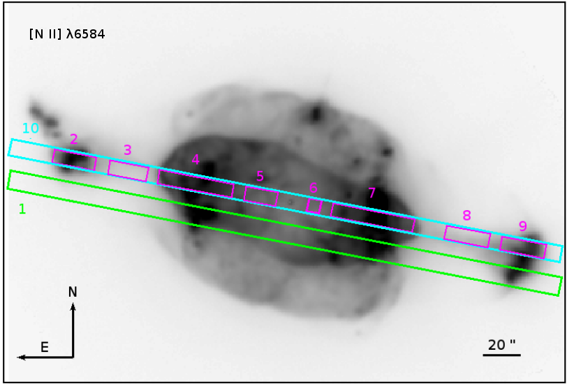
Fig. 8. Ten selected regions in NGC 7009 overlaid on the [N II] 6584A image. The position of the centre (x, y coordinates), position angle, width and length of the slits are free parameters provided by the user. Slits 1 and 10 represent the slits position from and , respectively. Numbered regions from 2 to 9 correspond to the sub-structures of knots and jet-like, or sub-regions of rims defined in [3].

Satellite calculates the H(beta) flux, line intensities (normalized to Hb=100 and corrected for interstellar extinction), emission line ratios (from the output.txt file), nebular parameters (Te, Ne), ionic/total elemental abundances, ICFs and abundance ratios for all 10 pseudo-slits. This module is executed from the specificPA_line_fluxes_script. The scripts slit_line_flux_script is employed in this module for each pseudo-slit.

c(H(beta)), emission line intensities and line ratios are saved in the output_linesintensities_per_angles.txt and output_lineratios_per_angles.txt files, respectively. So, the user can also perform any extra analysis he/she wants. Similarly, Te and Ne parameters are computed in the TeNe_specific_slits_script and are saved in the PyNeb_output_Te_and_Ne_specific_slits file, the ionic abundances are computed in the ionicabundances_specific_slits_script and are saved in the PyNeb_output_ionic_abund_specific_slits file, finally and the elemental abundances, ICFs and abundance ratios are computed in the element_abundances_ICFs_specific_slits_script and are saved in the PyNeb_output_total_abund_ICFs_specific_slits file.

Figure 8 shows the position of the specific areas/regions selected for the study of NGC 7009 overlaid on the [N II] flux map. The selected regions are the same as those defined by Goncalves et al. (2003) for a direct comparison of the results from the specific_slit_analysis module with 1D long-slit spectroscopic data. Possible differences between the two studies can be associated with the position of the pseudo-slits. At this point, it is worth mentioning the slit_position_testing module of the satellite code. This module is used to verify the position of the pseudo-slits before use the software. Hint: When the slit_position_testing module is used first deselect all other modules. Moreover, at least an emission line has to be used and defined in the input.txt file in order to properly use this module (e.g., Halpha) and Hbeta to avoid multiple maps). The output of this module is 10 figures (in png and pdf formats) with the position of each pseudo-slit overlaid on the emission line map (see Figure 9).

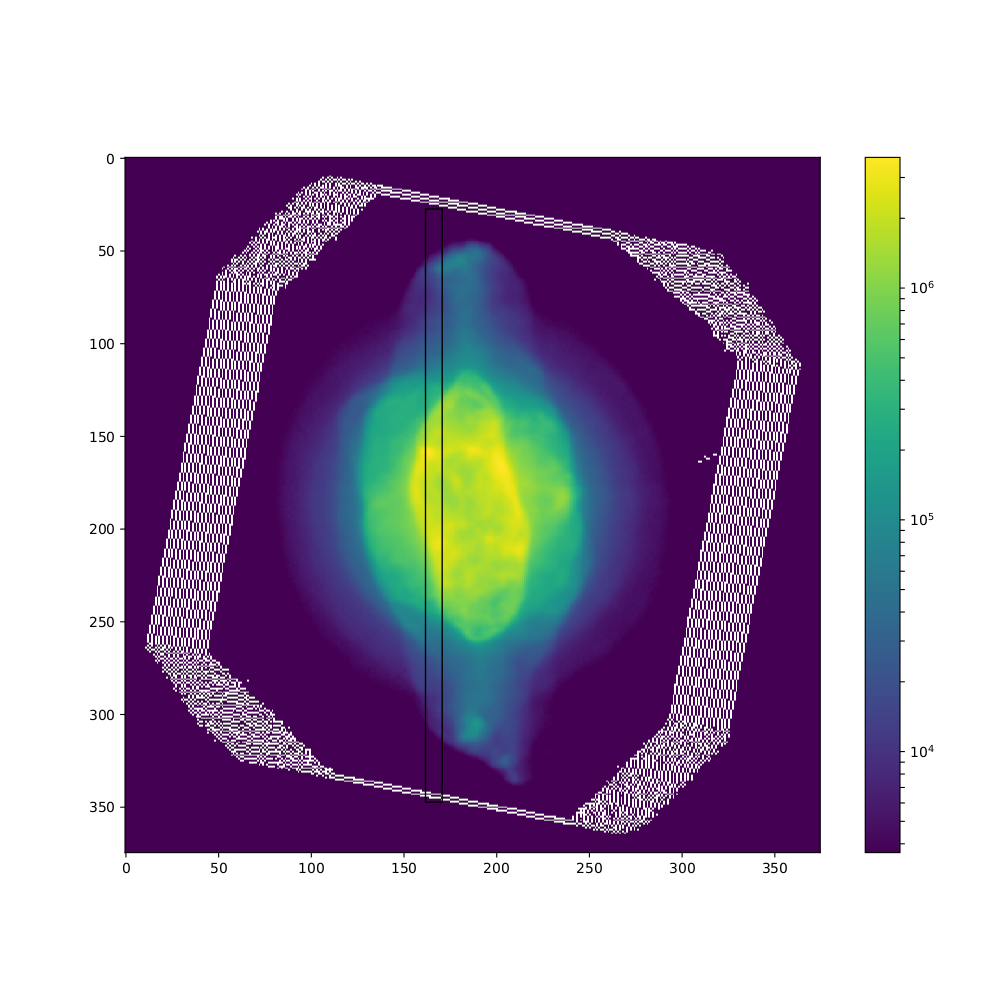
Fig. 9. Representative examples of the output figures produced by the slit_position_testing module. The slit from (left panel) and R1 slit from (right panel) are shown overlaid on the H(alpha) emission line maps. Scale is in "python counting; usual pixel counting starts in 1.](fig_slit0.pdf)

2D analysis module

Besides the 1D spectroscopic analysis, satellite also performs a spectroscopic analysis in both spatial dimensions simultaneously using the entire maps. For this module, the analysis2D_script, TeNe_2D_script, generate_2D_lineratio_maps_script, ionicabundances_2D_script, element_abundances_ICFs_2D_script and diagnotic_diagrams_script are employed.

c(Hbeta), line intensities, line ratios, Te, Ne, ionic, elemental abundances, ICFs and abundances ratios are computed for each individual pixels, if the criteria F(Ha)>0, F(Hb) > 0 and F(Ha) > F(Hb)*2.86 are satisfied, otherwise a value equals to "zero" is applied.

The main outcomes from this module are 2D maps for all the aforementioned nebular parameters saved in the output_images folder. In Figures 10, 11 and 12, the maps of c(Hbeta), Te and Ne using the [S III] and [S II] diagnostic lines, the line ratios log([N II]/[O III]) and log([S II]/S III]) are presented as representative examples of the outcomes from this module.

The 2D_spectroscopic_analysis module also calculates and returns the distribution of each maps (histogram plots), e.g., c(H(\beta)), Ne and Te maps (see Figures 12 and 13) as well as emission line diagnostic diagrams (see Figures 15 and 16) using the diagnotic_diagrams_script which are selected by the user in the diagnostic_diagrams_input file (see Figure 17).

Note1: At this point, it has to be clarified that when the specific_slits_analysis and/or rotation_analysis modules are used together with the 2D_analysis module, the emission lines ratios for the three modules are plotted on the same diagnostic diagrams for a direct comparison between an 1D and 2D analysis.

Last but not least, satellite computes and returns an ASCII file with the mean value, standard deviation and the percentiles of 5%, 25% (Q1), 50% (median), 75% (Q3), 95% for all the nebular parameters and emission line ratios for a thorough statistical analysis of the observed nebula.

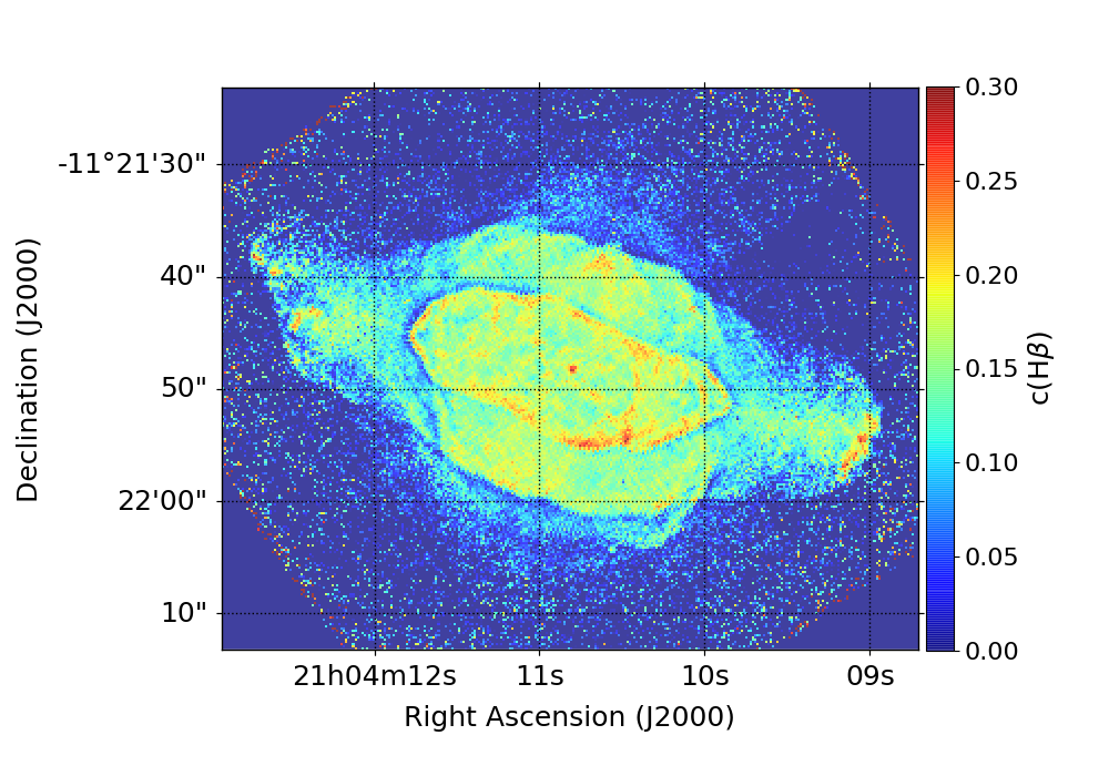
Fig. 10. c(H(beta) map of NGC 7009.

Fig. 11. Ne and Te maps obtained from the [S II] and [S III] diagnostic lines of NGC 7009.

Fig. 12. Log([N II]/[O III]) and log([S II]/[S III]) line ratio maps of NGC 7009

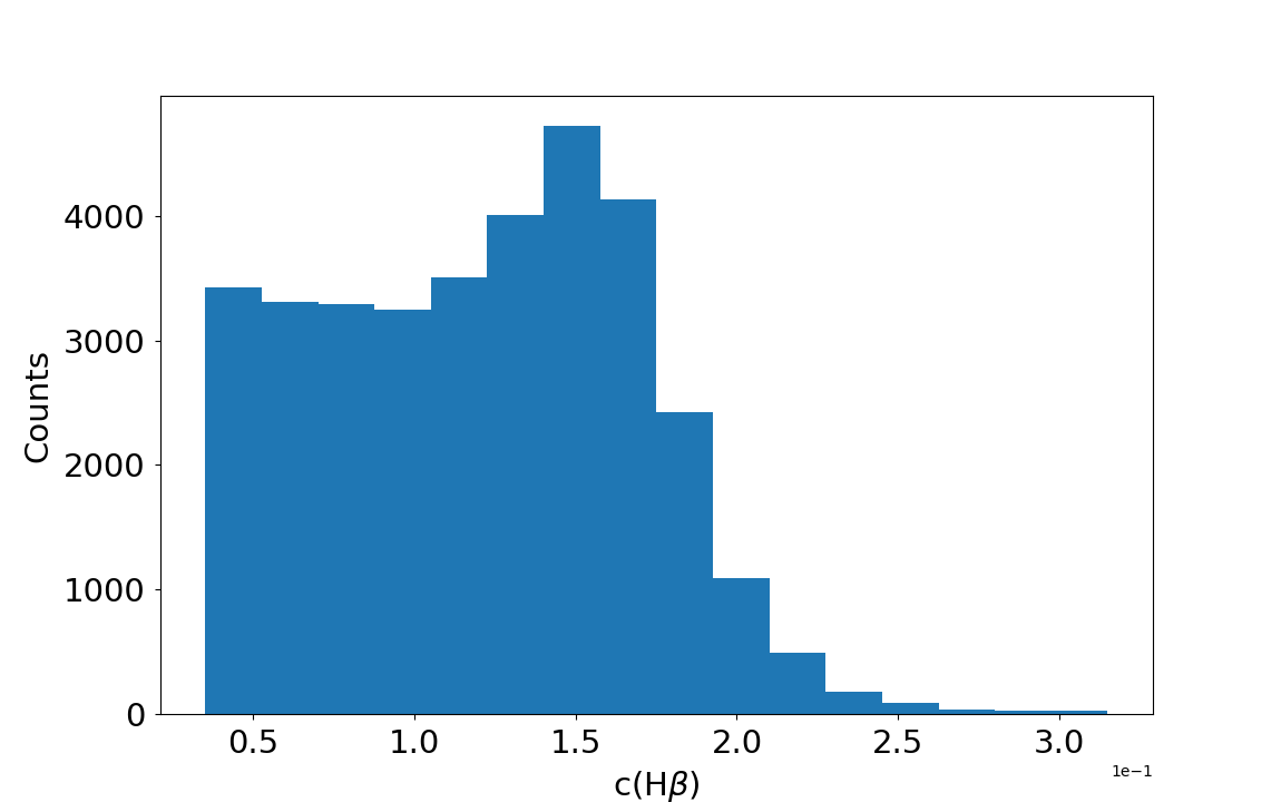
Fig. 13. The histogram of c(H(beta) map.

Fig. 14. The histograms of Ne[S II] and Te[S III] maps.

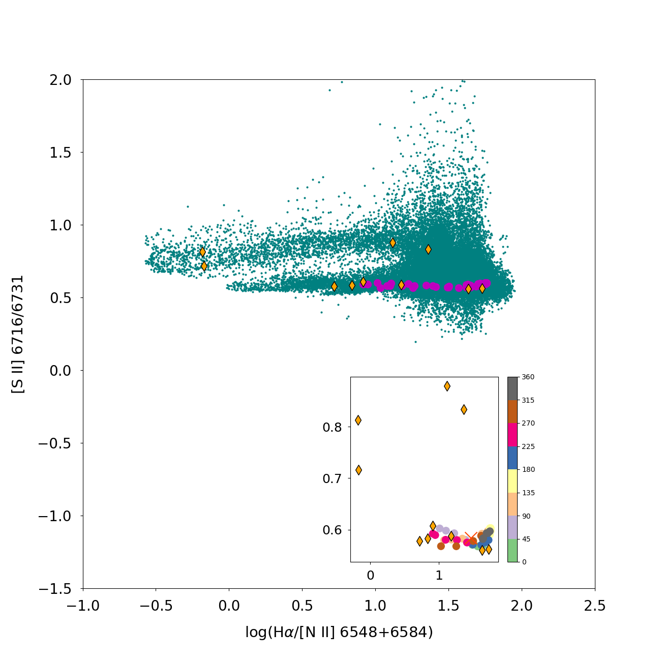
Fig. 15. A representative example of emission line diagnostic diagram: [S II] 6716/6731 versus H(alpha)/[N II] 6548+6584. Cyan dots correspond to the values of individual pixels, pink circles and yellow diamonds show the values obtained from the simulated long-slits of the rotational analysis task with position angles from 0 to 360 degrees with 10 degrees step and the values from the 10 simulated slits in the specific slits task, respectively. The inset plot illustrate the variation of the line ratios with the position angle of the simulated slits.

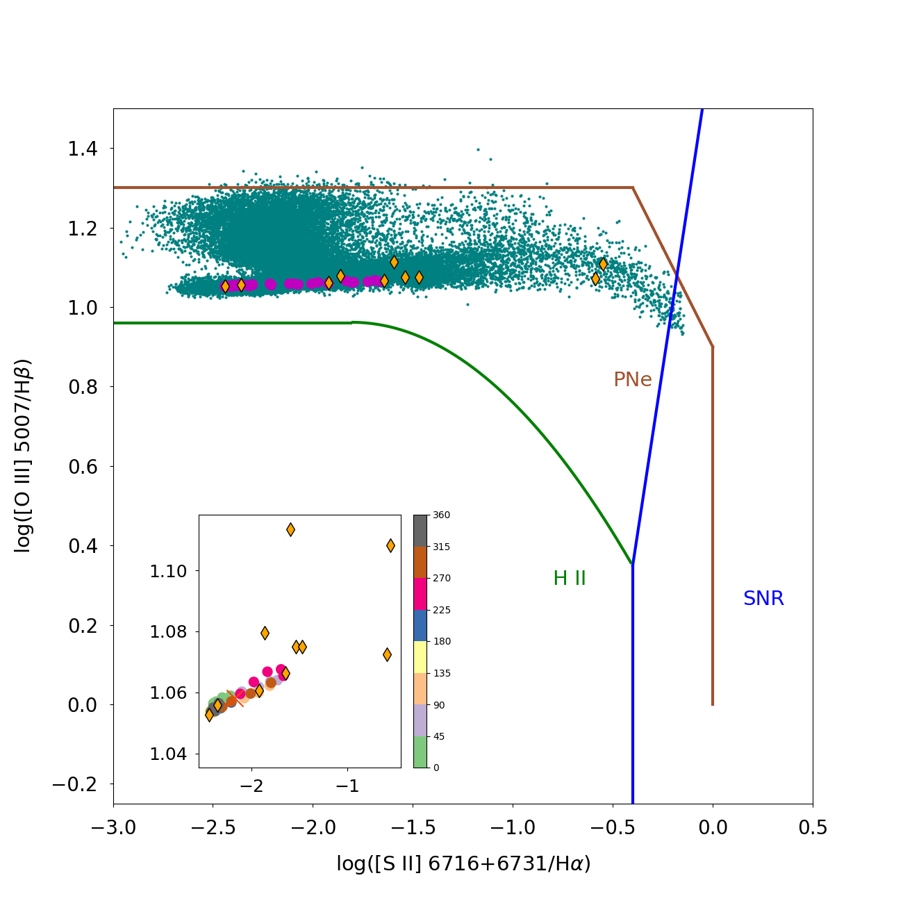
Fig. 16. A representative example of emission line diagnostic diagram: [O III] 5007/H(beta) versus [S II] 6716+6731/H(alpha). Cyan dots correspond to the values of individual pixels, pink circles and yellow diamonds show the values obtained from the simulated long-slits of the rotational analysis task with position angles from 0 to 360 degrees with 10 degrees step and the values from the 10 simulated slits in the specific slits task, respectively. The inset plot illustrate the variation of the line ratios with the position angle of the simulated slits. The regimes of the PNe, H ii regions and supernova remnants are also drawn.

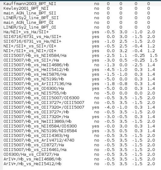
Fig. 17. An example of the diagnostic_diagrams_input.txt file for NGC 7009 and the parameters that the user can select for the diagnostic diagrams in the 2D_analysis_module module.

radial analysis module

The final module in the current version of satellite (v1.3) conducts a radial spectroscopic analysis considering a pseudo-slit with specific width, length and position angle (parameter=angle_for_radial_flux) provided by the user in the numerical_input.txt file. The user must also select the emission lines that will be used for this analysis. This can be made in the third column of the input.txt file: radial_yes, or radial_no.

Note1: It is recommended to disable all other modules when the radial_analysis module is executed. The main outcomes of this module are:

(I) the radial profiles of all the selected emission lines in the input.txt normalized by the peak flux.
(II) the calculation of all the nebular parameters (c(H(beta)), line intensities, line ratios, Te, Ne, ionic, elemental abundances, ICFs and abundances ratios) as functions of the distance from the central star or the central point of the nebula or galaxy in general.

The normalization of the radial profiles is made using the peak of the flux of each emission line. However, the user can also select the range from where this peak can be obtained by providing the code with the minimum radius (limit_radial_in_arcsec parameter). This option permit to investigate the radial distribution of emission lines for regions/substructures with specific interest.

The radial profile of various emission lines for the example of NGC 7009 are shown in Figure 18 (Hint: It is recommended to use maximum 4-6 lines for the construction of more illustrative plots.). All radial profiles are normalized to a peak flux found for distances r(>)20 arcsec (_radial_in_arcsec > 20) focused to the low-ionization structures/knot of NGC 7009. The calculation are made in the find_maxvlaue_script. Hence, satellite returns the distance between the peak of each selected line and the central star in arcsec. Table 1 lists the distances for the example of NGC 7009 and it can be seen that there is a spatial offset of 1 arcsec between the high/moderate- and low-ionization lines. The values of each radial step (pixel scale of the IFU) are also saved in an ASCII file, so the user can build his/her own radial profiles.

The radial variation of c(H(beta)), Te, and Ne parameters of NGC 7009 are shown in Figure 19.

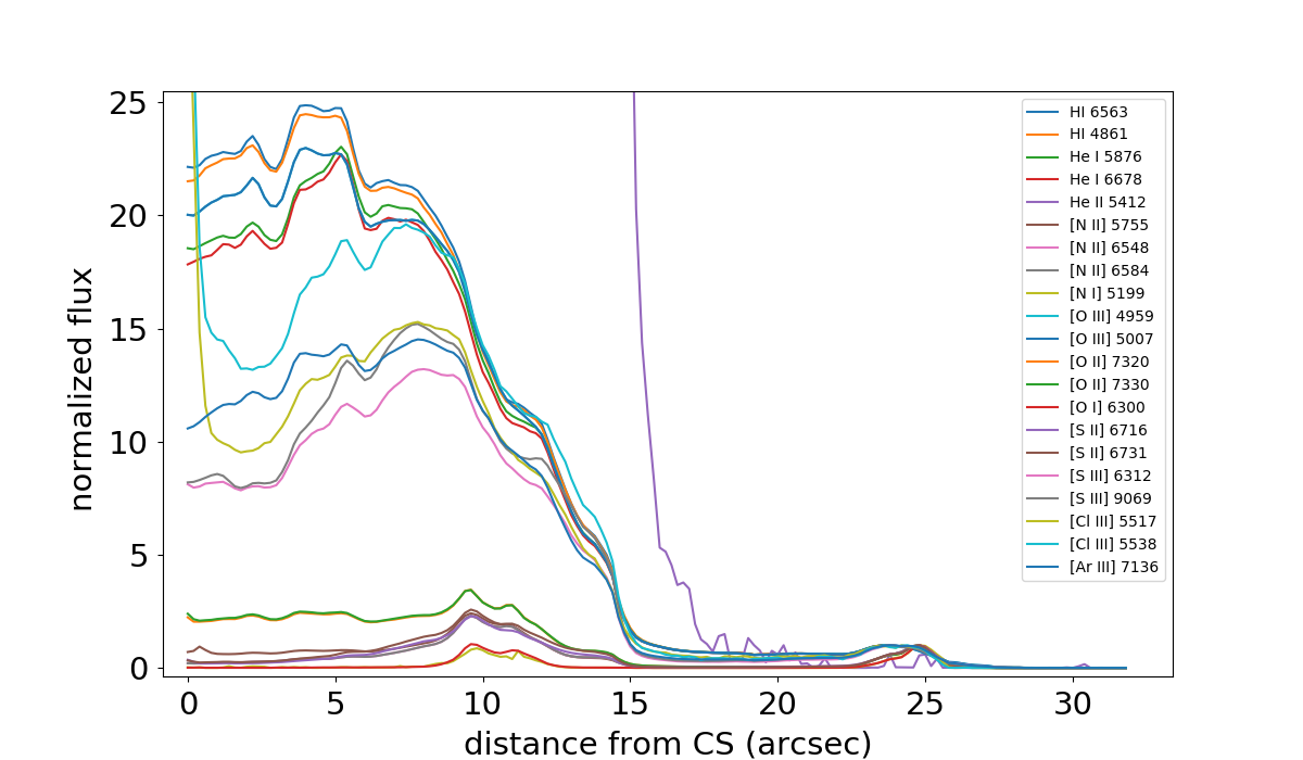
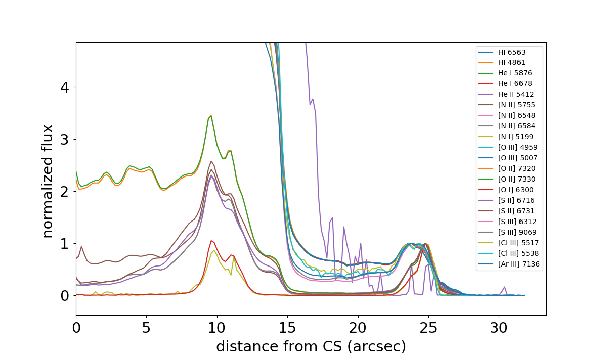
Fig. 18. Radial profiles for several emission lines of NGC 7009 at PA=79 degrees. Upper panel shows all the radial profiles, while the lower panel zooms-in to the much fainter emission lines.

Fig. 19. Representative examples of the radial distribution of c(H(beta)) upper panel and Te, Ne (lower panel).

One again, it has to be pointed out that the code sums up the values of the pixels which have F(Halpha>0, F(Hbeta)>0 and/or F(Halpha)>F(Hbeta)*2.86.


Line	distance (a)	Line	distance
	(arcsec)		(arcsec)
H I 4861	23.6	[N II] 6548	24.8
[O III] 4959	23.8	H I 6563	23.6
[N I] 5199	24.8	[N II] 6584	24.8
He II 5412	20.2	He I 6678	23.8
[Cl III] 5517	24.2	[S II] 6716	24.8
[Cl III] 5538	24.4	[S II] 6731	24.8
[N I] 5755	24.2	[Ar III] 7136	24.8
He I 5876	23.6	[O II] 7320	24.8
[O II] 6300	24.8	[O II] 7330	24.8
[S III] 6312	23.8	[S III 9069	23.8

Distances from the central stars of emission line's peak for a pseudo-slit at 79 degree position angle

(a) The spacial resolution of MUSE maps is 0.2 arcsec.

radial distance calculations

At this point, it is necessary to further explain how satellite calculates the fluxes of the emission lines as function of the distance from the central star. Figure 20 shows an example of a pseudo-slit at PA=90 degrees.

The width of the pseudo-slit defines how many pixels will be taken into consideration for the flux at each distance. For instance, the fluxes (and errors) of 5 pixels are summed up for the first column (or radial distance r=0.2 arcsec). Then, the code moves to the second column and computes the flux and the corresponding error from the next 5 pixels at the radial distance r=0.4 arcsec and so on (see Figure 20).

After finishing the computation of the fluxes and errors for all the lines, the code computes the extinction coefficient (c(H(\beta))) and corrected line intensities (relative to H(beta)=100) as function of the radial distance from the central star or geometric centre as well as all nebular parameters (Te, Ne, ionic, elemental abundances, ICFs and abundance ratios) (Figures 18 and 19).

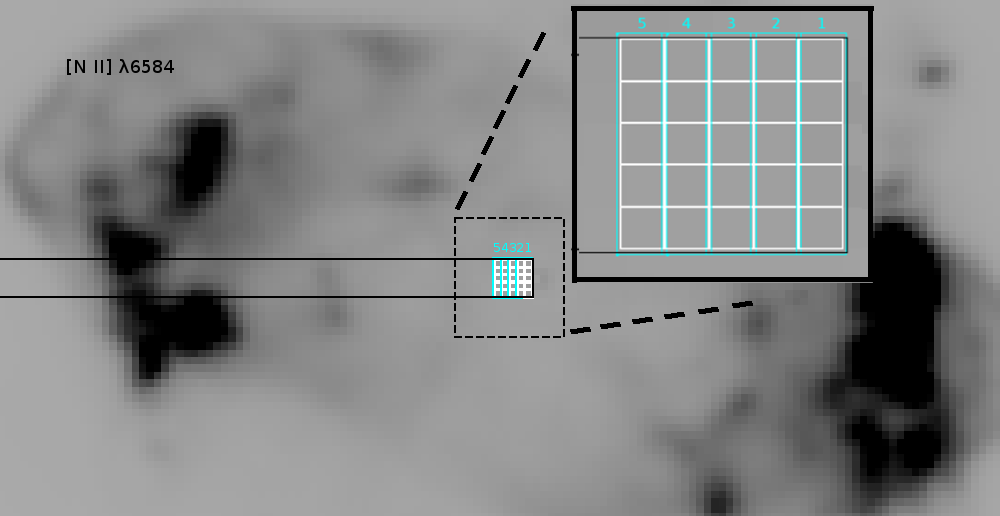
Fig. 20. An illustrative example of how satellite computes the fluxes and radial stances from the central star of the nebula or the geometric centre of the nebula.

Uncertainty calculations

The uncertainties of emission lines and all nebular parameters for all four modules are computed following the same Monte Carlo approach. In particular, satellite, first, computes the total error of the flux for each pseudo-slit or pixel, using the provided error maps + an extra error as the percentage of the flux.

[\Delta F_{tot}=\Sigma_{i=1}^{N}~(\sigma_{F_i}+\lambda*F_i)^{1/2}]

where i corresponds to the pseudo-slit or pixel and range from 1 to the total number N, (\sigma_{F_i}) is the uncertainties of the flux in the pseudo-slit or pixel i based on the provided error maps, F(_i) is the flux in the pseudo-slit or pixel i and (\lambda) corresponds to the percentage of the flux (from 0 to 1.0). If (\lambda)=0, then the code takes into account only the errors from the maps. The (\lambda)=0 parameter is given to the code by the user in the input.txt file (forth column). There is also the option not to use the error maps. This is defined in the input.txt file (forth column) even rows (the rows of errors). If a non-zero value is provided, the code uses the formula (1) while for a "0" value , the code uses the formula (2).

[\Delta F_{tot}=\Sigma_{i=1}^{N}~(\lambda*F_i)^{1/2}]

These resultant uncertainties of the line fluxes are then used to replicate the spectrum of a pseudo-slit or pixel, and a number of additional spectra are generated using a Monte Carlo algorithm. The number of the replicate spectra is given by the user in the numerical_input.txt. satellite computes all the nebular parameters, e.g. Te, Ne, ionic, elemental abundances and ICFs for all the replicate spectra and the standard deviation of each parameters is the uncertainty of the parameter that the satellite code provides.

General Notes:

It has to be clarified that the satellite code takes as input a list of emission line fluxes and error maps extracted from the datacubes obtained from any IFU. It does not extract the maps from the datacudes. Therefore, this is a step that has to be done before the use of satellite.
Moreover, satellite can also be applied to individual emission lines images obtained with narrow band filters (if there are available) or the emission line images obtained from 3D photo-ionization models.

Possible error messages

In this section, a number of possible errors that may come out are described.

In case an emission line is missing, the user has to define that in the input.txt file by writing "no" in the second and third columns of the corresponding line. If the user has forgotten to properly change the output.txt file or the diagnostic_diagram_input.txt file, an error will be return, see Figure 21.
In case an emission line is missing, but the user has forgotten to properly change the output.txt file or the diagnostic_diagram_input.txt file and a physical parameters has to be computed such as Te, Ne, abundances, an error will be return like in Figure 22.
In case, the arrays of the emission lines have different sizes an error will be return like in Figure 23. Moreover, the error line may also be related to the parameters total_num_pixels_verti and total_num_pixels_horiz in the numerical_input.txt file.

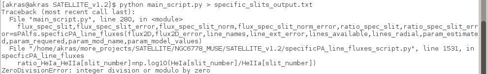
Fig. 21. An example of error in case the He II line is missing (in the input.txt file, it has been set as "no") but the He I/He II ratio is required to be computed (in the output.txt, the He I/He II ratio is still "yes").

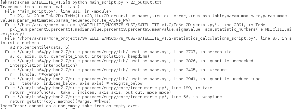
Fig. 22. An example of error in case a physical parameter is required to be computed and the corresponding line is missing (in the input.txt file, it has been set as "no". In this example, the Te and Ne from the [N II] and [Cl III] diagnostic lines have to be computed but a diagnostic line is missing.

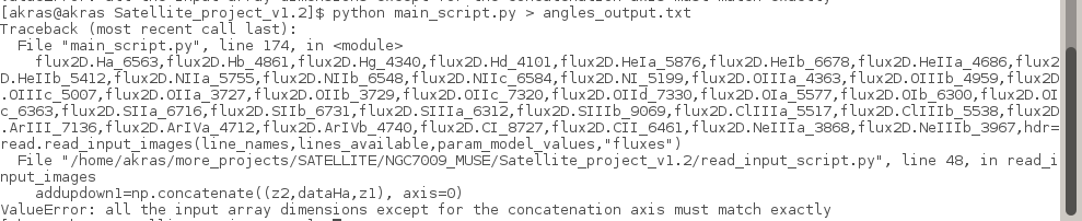
Fig. 23. An example of error in case there is a problem with the dimensions of the arrays that correspond to the emission lines. In this case, the error is because the size of the flux maps is not consistent with the total_num_pixels_verti and total_num_pixels_horiz parameters in the numerical_input.txt file.

How to Cite satellite in a publication?

There are two papers appropriate as references for satellite in a publication. They are:
1) Akras, Stavros; Monteiro, Hektor; Aleman, Isabel; Farias, Marcos A. F. ; May, Daniel ; Pereira, Claudio B., 2020, MNRAS, 493, 2238A

bibtex code:
@ARTICLE2020MNRAS.493.2238A,
author = Akras, Stavros and Monteiro, Hektor and Aleman, Isabel and Farias, Marcos A. F. and May, Daniel and Pereira, Claudio B.,
title = "Exploring the differences of integrated and spatially resolved analysis using integral field unit data: the case of Abell 14",
journal = (\setminus)mnras,
keywords = techniques: imaging spectroscopy; techniques: spectroscopic; (stars:) binaries: general, ISM: abundances, (ISM:) planetary nebulae: individual: Abell 14, Astrophysics - Astrophysics of Galaxies, Astrophysics - Solar and Stellar Astrophysics,
year = 2020,
month = apr,
volume = 493,
number = 2,
pages = 2238-2252,
doi = 10.1093/mnras/staa383,
archivePrefix = arXiv,
eprint = 2002.12380,
primaryClass = astro-ph.GA,
adsurl = https://ui.adsabs.harvard.edu/abs/2020MNRAS.493.2238A,
adsnote = Provided by the SAO/NASA Astrophysics Data System

2) S. Akras; H. Monteiro; J. R. Walsh; J. García-Rojas; I. Aleman; H. Boffin; P. Boumis; A. Chiotelis; R. M. L. Corradi; D. R. Gonçalves; L. A. Gutiérrez-Soto; D. Jones; C. Morisset, 2021, MNRAS, submitted

Licence and Copyright Information

satelite is freely available under the General Public License (GPL).

Questions of problems

For questions please write an email to Dr. Stavros Akras ([email protected])

stavrosakras / satellite Goto Github PK

satellite's Introduction