

This REANA reproducible analysis example studies the Higgs-to-four-lepton decay channel that led to the Higgs boson experimental discovery in 2012. The example uses CMS open data released in 2011 and 2012. "This research level example is a strongly simplified reimplementation of parts of the original CMS Higgs to four lepton analysis published in Phys.Lett. B716 (2012) 30-61, arXiv:1207.7235." (See Ref. 1).
Making a research data analysis reproducible basically means to provide "runnable recipes" addressing (1) where is the input data, (2) what software was used to analyse the data, (3) which computing environments were used to run the software and (4) which computational workflow steps were taken to run the analysis. This will permit to instantiate the analysis on the computational cloud and run the analysis to obtain (5) output results.
The analysis takes the following inputs:
- the list of CMS validated runs included in the
datadirectory:Cert_190456-208686_8TeV_22Jan2013ReReco_Collisions12_JSON.txt
- a set of data files in the ROOT format, processed
from CMS public datasets, included in the
datadirectory:DoubleE11.rootDoubleE12.rootDoubleMu11.rootDoubleMu12.rootDY1011.rootDY1012.rootDY101Jets12.rootDY50Mag12.rootDY50TuneZ11.rootDY50TuneZ12.rootDYTo2mu12.rootHZZ11.rootHZZ12.rootTTBar11.rootTTBar12.rootTTJets11.rootTTJets12.rootZZ2mu2e11.rootZZ2mu2e12.rootZZ4e11.rootZZ4e12.rootZZ4mu11.rootZZ4mu12.root
- CMS collision data from 2011 and 2012 accessed "live" during analysis via CERN Open Data portal:
- CMS simulated data from 2011 and 2012 accessed "live" during analysis via CERN Open Data portal:
"The example uses legacy versions of the original CMS data sets in the CMS AOD, which slightly differ from the ones used for the publication due to improved calibrations. It also uses legacy versions of the corresponding Monte Carlo simulations, which are again close to, but not identical to, the ones in the original publication. These legacy data and MC sets listed below were used in practice, exactly as they are, in many later CMS publications.
Since according to the CMS Open Data policy the fraction of data which are public (and used here) is only 50% of the available LHC Run I samples, the statistical significance is reduced with respect to what can be achieved with the full dataset. However, the original paper Phys.Lett. B716 (2012) 30-61, arXiv:1207.7235, was also obtained with only part of the Run I statistics, roughly equivalent to the luminosity of the public sets, but with only partial statistical overlap."(See Ref. 1).
The analysis will consist of three stages. In the first stage, we shall build
the analysis code plugin for the CMSSW analysis
framework, contained in the HiggsDemoAnalyzer directory, using
SCRAM, the official
CMS software build and management tool. In the second stage, we shall process
the original collision data (using demoanalyzer_cfg_level3data.py
) and simulated data (using demoanalyzer_cfg_level3MC.py
) for one Higgs signal candidate with with reduced statistics. In the third
and final stage, we shall plot the results (using M4Lnormdatall_lvl3.cc).
"The provided analysis code recodes the spirit of the original analysis and recodes many of the original cuts on original data objects, but does not provide the original analysis code itself. Also, for the sake of simplicity, it skips some of the more advanced analysis methods of the original paper. Nevertheless, it provides a qualitative insight about how the original result was obtained. In addition to the documented core results, the resulting root files also contain many undocumented plots which grew as a side product from setting up this example and earlier examples. The significance of the Higgs 'excess' is about 2 standard deviations in this example, while it was 3.2 standard deviations in this channel alone in the original publication. The difference is attributed to the less sophisticated background suppression. In more recent (not yet public) CMS data sets with higher statistics the signal is observed in a preliminary analysis with more than 5 standard deviations in this channel alone CMS-PAS-HIG-16-041.
The analysis strategy is the following: Get the 4mu and 2mu2e final states from the DoubleMuParked datasets and the 4e final state from the DoubleElectron dataset. This avoids double counting due to trigger overlaps. All MC contributions except top use data-driven normalization: The DY (Z/gamma^*) contribution is scaled to the Z peak. The ZZ contribution is scaled to describe the data in the independent mass range 180-600 GeV. The Higgs contribution is scaled to describe the data in the signal region. The (very small) top contribution remains scaled to the MC generator cross section." (See Ref. 1).
In order to be able to rerun the analysis even several years in the future, we need to "encapsulate the current compute environment", for example to freeze the software package versions our analysis is using. We shall achieve this by preparing a Docker container image for our analysis steps.
This analysis example runs within the CMSSW analysis framework that was packaged for Docker in docker.io/cmsopendata/cmssw_5_3_32.
The analysis workflow is simple and consists of three above-mentioned stages:
                           START
                             |
                             |
                             V
               +-------------------------+
               |           SCRAM         |
               +-------------------------+
                          /     \
                         /       \
                        /         \
+-------------------------+     +------------------------+
| process collision data  |     | process simulated data |
+-------------------------+     +------------------------+
                \                       /
                 \ Higgs4L1file.root   / DoubleMuParked2012C_10000_Higgs.root
                  \                   /
               +-------------------------+
               |    produce final plot   |
               +-------------------------+
                          |
                          | mass4l_combine_userlvl3.pdf
                          V
                         STOP
The steps processing collision data and simulated data can be run in parallel. We shall use the Snakemake workflow specification to express the computational workflow by means of the following Snakefile:
rule all:
    input:
        "results/mass4l_combine_userlvl3.pdf"

rule scram:
    input:
        config["data"],
        config["code"]
    output:
        touch("results/scramdone.txt")
    container:
        "docker://docker.io/cmsopendata/cmssw_5_3_32"
    shell:
        "source /opt/cms/cmsset_default.sh "
        "&& scramv1 project CMSSW CMSSW_5_3_32 "
        "&& cd CMSSW_5_3_32/src "
        "&& eval `scramv1 runtime -sh` "
        "&& cp -r ../../code/HiggsExample20112012 . "
        "&& cd HiggsExample20112012/HiggsDemoAnalyzer "
        "&& scram b "
        "&& cd ../Level3 "
        "&& mkdir -p ../../../../results "

rule analyze_data:
    input:
        config["data"],
        config["code"],
        "results/scramdone.txt"
    output:
        "results/DoubleMuParked2012C_10000_Higgs.root"
    container:
        "docker://docker.io/cmsopendata/cmssw_5_3_32"
    shell:
        "source /opt/cms/cmsset_default.sh "
        "&& cd CMSSW_5_3_32/src "
        "&& eval `scramv1 runtime -sh` "
        "&& cd HiggsExample20112012/HiggsDemoAnalyzer "
        "&& cd ../Level3 "
        "&& cmsRun demoanalyzer_cfg_level3data.py"

rule analyze_mc:
    input:
        config["data"],
        config["code"],
        "results/scramdone.txt"
    output:
        "results/Higgs4L1file.root"
    container:
        "docker://docker.io/cmsopendata/cmssw_5_3_32"
    shell:
        "source /opt/cms/cmsset_default.sh "
        "&& cd CMSSW_5_3_32/src "
        "&& eval `scramv1 runtime -sh` "
        "&& cd HiggsExample20112012/HiggsDemoAnalyzer "
        "&& cd ../Level3 "
        "&& cmsRun demoanalyzer_cfg_level3MC.py"

rule make_plot:
    input:
        config["data"],
        config["code"],
        "results/DoubleMuParked2012C_10000_Higgs.root",
        "results/Higgs4L1file.root"
    output:
        "results/mass4l_combine_userlvl3.pdf"
    container:
        "docker://docker.io/cmsopendata/cmssw_5_3_32"
    shell:
        "source /opt/cms/cmsset_default.sh "
        "&& cd CMSSW_5_3_32/src "
        "&& eval `scramv1 runtime -sh` "
        "&& cd HiggsExample20112012/HiggsDemoAnalyzer "
        "&& cd ../Level3 "
"&& root -b -l -q ./M4Lnormdatall_lvl3.cc"The example produces a plot showing the now legendary Higgs signal:
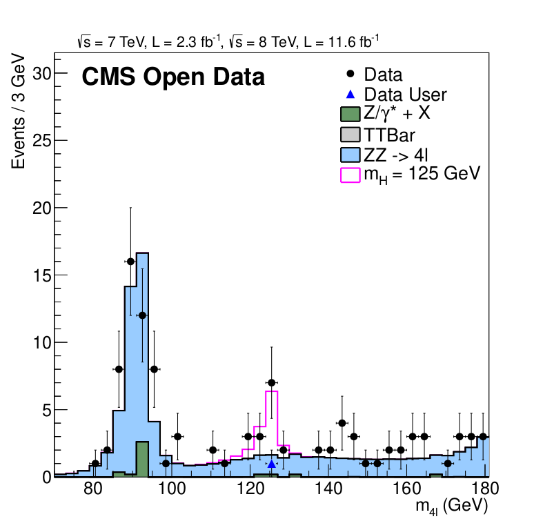
The published reference plot which is being approximated in this example is https://inspirehep.net/record/1124338/files/H4l_mass_3.png. Other Higgs final states (e.g. Higgs to two photons), which were also part of the same CMS paper and strongly contributed to the Higgs boson discovery, are not covered by this example.
There are two ways to execute this analysis example on REANA.
If you would like to simply launch this analysis example on the REANA instance at CERN and inspect its results using the web interface, please click on the following badge:
If you would like a step-by-step guide on how to use the REANA command-line client to launch this analysis example, please read on.
We start by creating a reana.yaml file describing the above analysis structure with its inputs, code, runtime environment, computational workflow steps and expected outputs. In this example we are using the Snakemake workflow specification, which you can find in the workflow directory.
We can now install the REANA command-line client, run the analysis and download the resulting plots:
$ # create new virtual environment
$ virtualenv ~/.virtualenvs/myreana
$ source ~/.virtualenvs/myreana/bin/activate
$ # install REANA client
$ pip install reana-client
$ # connect to some REANA cloud instance
$ export REANA_SERVER_URL=https://reana.cern.ch/
$ export REANA_ACCESS_TOKEN=XXXXXXX
$ # create new workflow
$ reana-client create -n my-analysis
$ export REANA_WORKON=my-analysis
$ # upload input code and data to the workspace
$ reana-client upload
$ # start computational workflow
$ reana-client start
$ # ... should be finished in a couple (~5) of minutes
$ reana-client status
$ # list workspace files
$ reana-client list
$ # download output results
$ reana-client download
Please see the REANA-Client
documentation for more detailed explanation of typical reana-client usage
scenarios.
This example is based on the original open data analysis by Jomhari, Nur Zulaiha; Geiser, Achim; Bin Anuar, Afiq Aizuddin, "Higgs-to-four-lepton analysis example using 2011-2012 data", CERN Open Data Portal, 2017. DOI: 10.7483/OPENDATA.CMS.JKB8.RR42
The list of contributors to this REANA example in alphabetical order:


