jakevdp / nfft Goto Github PK

Lightweight non-uniform Fast Fourier Transform in Python

License: MIT License

Jupyter Notebook 82.58% Makefile 0.10% Python 17.31%

nfft's Introduction

nfft package

The nfft package is a lightweight implementation of the non-equispaced fast Fourier transform (NFFT), implemented via numpy and scipy and released under the MIT license. For information about the NFFT algorithm, see the paper Using NFFT 3 – a software library for various nonequispaced fast Fourier transforms.

The nfft package achieves comparable performance to the C package described in that paper, without any customized compiled code. Rather, it makes use of the computational building blocks available in NumPy and SciPy. For a discussion of the algorithm and this implementation, see the Implementation Walkthrough notebook.

About

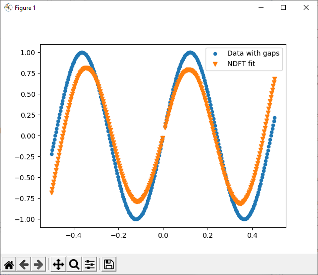
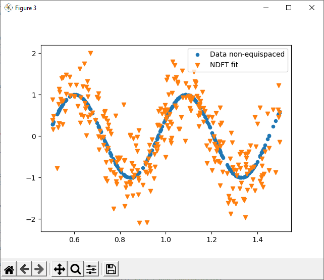
The nfft package implements one-dimensional versions of the forward and adjoint non-equispaced fast Fourier transforms;

The forward transform:

$f_j = \sum_{k=-N/2}^{N/2-1} \hat{f}_k e^{-2\pi i k x_j}$

And the adjoint transform:

$\hat{f}k = \sum{j=0}^{M-1} f_j e^{2\pi i k x_j}$

In both cases, the wavenumbers k are on a regular grid from -N/2 to N/2, while the data values x_j are irregularly spaced between -1/2 and 1/2.

The direct and fast version of these algorithms are implemented in the following functions:

nfft.ndft: direct forward non-equispaced Fourier transform
nfft.nfft: fast forward non-equispaced Fourier transform
nfft.ndft_adjoint: direct adjoint non-equispaced Fourier transform
nfft.nfft_adjoint: fast adjoint non-equispaced Fourier transform

Computational complexity

The direct version of each transform has a computational complexity of approximately O[NM], while the NFFT has a computational complexity of approximately O[N log(N) + M log(1/ϵ)], where ϵ is the desired precision of the result. In the current implementation, memory requirements scale as approximately O[N + M log(1/ϵ)].

Comparison to pynfft

Another option for computing the NFFT in Python is to use the pynfft package, which provides a Python wrapper to the C library referenced in the above paper. The advantage of pynfft is that, compared to nfft, it provides a more complete set of routines, including multi-dimensional NFFTs, several related extensions, and a range of computing strategies.

The disadvantage is that pynfft is GPL-licensed (and thus can't be used in much of the more permissively licensed Python scientific world), and has a much more complicated set of dependencies.

Performance-wise, nfft and pynfft are comparable, with the implementation within nfft package being up to a factor of 2 faster in most cases of interest (see Benchmarks.ipynb for some simple benchmarks).

If you're curious about the implementation and how nfft attains such performance without a custom compiled extension, see the Implementation Walkthrough notebook.

Basic Usage

import numpy as np
from nfft import nfft

# define evaluation points
x = -0.5 + np.random.rand(1000)

# define Fourier coefficients
N = 10000
k = - N // 2 + np.arange(N)
f_k = np.random.randn(N)

# non-equispaced fast Fourier transform
f = nfft(x, f_k)

For some more examples, see the notebooks in the notebooks directory.

Installation

The nfft package can be installed directly from the Python Package Index:

$ pip install nfft

Dependencies are numpy, scipy, and pytest, and the package is tested in Python versions 2.7. 3.5, and 3.6.

Testing

Unit tests can be run using pytest:

$ pytest --pyargs nfft

License

This code is released under the MIT License. For more information, see the Open Source Initiative

Support

Development of this package is supported by the UW eScience Institute, with funding from the Gordon & Betty Moore Foundation, the Alfred P. Sloan Foundation, and the Washington Research Foundation

nfft's People

Contributors

Stargazers

Watchers

nfft's Issues

Why I get an assertion error in this example

I have a signal r which was evaluated(sampled) at time t and the sampling frequency is not constant. The data are:

r = np.array([119.78410766, 119.76753142, 117.62636578, 103.44442714,
       100.20643576, 100.07845224, 100.8635375 , 105.7013656 ,
       115.19253386, 118.8410111 , 119.56967806, 119.49016405,
       115.673267  , 102.86539977, 100.18330076, 100.19053755,
       100.96717742, 104.64258496, 112.76883508, 118.42145725,
       119.46248759])

t = np.array([-408.60214685, -367.98645179, -326.11763398, -283.30427476,
       -240.51508415, -198.71111261, -158.2850487 , -118.96667683,
        -79.99044514,  -40.53604325,    0.        ,   41.86292241,
         84.76209664,  127.57962255,  169.0752062 ,  209.26407576,
        248.94525408,  288.63548604,  328.64737256,  369.17828499,
        410.49942551])

plt.plot(t, r, label='data')
plt.legend()

In the t variable the distance between each sampling instance is between 39 to 42 and not constant and this made the fft inaccurate for me.

When I use nfft however, I get the following assertion error but I am not sure what my mistake is in using the nfft package.

from nfft import nfft
f = nfft(z, r)

AssertionError Traceback (most recent call last)
in
1 from nfft import nfft
----> 2 f = nfft(z, r)

~/.local/share/virtualenvs/tf-tRAPLeXL/lib/python3.6/site-packages/nfft/core.py in nfft(x, f_hat, sigma, tol, m, kernel, use_fft, truncated)
123
124 N = len(f_hat)
--> 125 assert N % 2 == 0
126
127 sigma = int(sigma)

AssertionError:

ENH: add N-dimensional methods

Should be able to use the same csr-based summation scheme by flattening the [mxmxm...] block at each point/row.

Problems about Fourier operations and the inverse operations

Hi,
I'm not very sure how to define the inverse Fourier transforms. Is it the adjoint method?
Thank you.

What is the complexity of your implementation

Very nice package! I was wondering what the complexity is if your particular implementation. The 1D FFT is O(N*log(N)), I assume your algorithm depends on N, M and the accuracy eps. You can put this information in the README, I think it would be very useful to readers.

How to get dominating frequency of the signal

So my question is how can we get dominating frequency / frequencies from the signal?

That is sth I can achieve with scipy.FFTPACK using code like that:
import scipy.fftpack as syfp
X = syfp.fft(signal)
freqs = syfp.fftfreq(len(signal)) * SamplesPerSecond
dominatingFreqId= np.argsort(np.abs(X))[-1]
freq = freqs[dominatingFreqId]

How can I achieve that with NFFT, but of course on not equally spaced samples? I.e. it would be nice if I can get the frequency using code sample by jakevdp from this thread: #7

Frequency resolution of f_hat

Hi,

I have a question regarding the frequency resolution for the vector of Fourier coefficients.
No matter what I do, whether I use equal M and N, or one being a multiple of the other, it doe's not change the frequency resolution of the coefficients given in f_hat. For equidistant FFT, there is is a relationship for df, which is the reciprocal of M * dt. This obviously does not apply here, since df stays always at df = 1 Hz.
Is there a chance to change this behavior, or am I doing something wrong in principle?
Here is my little test to check the right frequencies and amplitudes. I can see that the 200 Hz, for example, is always at index 200.

import numpy as np
import nfft as nf

n = 2**13
dt = 1.0e-4

x = np.linspace(0.0, n*dt, n)
y = 2. * np.sin(2. * np.pi * 2.5 * x) + 0.5 * np.sin(2. * np.pi * 50. * x) + 1.25 * np.sin(2. * np.pi * 200. * x)

f_hat = nf.nfft_adjoint(x, y, n)

import matplotlib.pyplot as plt
plt.plot(2.0/n * np.abs(f_hat[n//2:]))

plt.grid()
plt.xlim(195, 205)

plt.savefig('test.png')

THX!
Patrick

Signal reconstruction outside the data range on which the nfft was calculated

Hi,

I did an experiment with the output of the nfft which I was not sure how to interpret it.
First I calculate the nfft_adjoint and then based on the output try to reconstruct the result which works.

N = 100000
K = -N / 2 + np.arange(N)
fk_hat = nfft.nfft_adjoint(z, r, N)

fk = 0
for i, k in enumerate(K):
    fk += fk_hat[i]*np.exp(-2*np.pi*1j*k*z)
    
plt.plot(z, fk/(N), '-', color='red', label='nfft')
plt.plot(z, r, '.', color='blue', label='data')
plt.legend()

Then I augment the input z to z3 and calculate the reconstruction on it:


z1 = np.linspace(-700,-422,20)
z2 = np.linspace(424,700, 20)
z3 = np.concatenate((z1, z, z2))

N = 100000
K = -N / 2 + np.arange(N)
fk_hat = nfft.nfft_adjoint(z, r, N)


fk = 0
for i, k in enumerate(K):
    fk += fk_hat[i]*np.exp(-2*np.pi*1j*k*z3)
    
plt.plot(z3, fk/(N), '-', color='red', label='nfft')
plt.plot(z, r, '.', color='blue', label='data')
plt.legend()

It is also the same output if I use the original forward fft.

N= 100000
k = -N / 2 + np.arange(N)
r_hat = nfft.nfft_adjoint(z, r, N)

r_reconstructed = nfft.nfft(z3, r_hat) / N
plt.plot(z, r, '.', color='blue')
plt.plot(z3, r_reconstructed, '-', color='red')

My expectation was to see also the same wave continue osculating outside the data range the adjoing nfft was calculated on it.

Isn't the purpose of nfft finding the true frequency components of a signal similar to fft, or have I been using it incorrectly.

my data is in addition as follows:

r = np.array([119.75024144, 119.77177673, 119.79671626, 119.81566188,
       119.81291201, 119.71610143, 119.24156708, 117.66932347,
       114.22145178, 109.27266933, 104.57675147, 101.63381325,
       100.42623807, 100.09436745, 100.02798438, 100.02696846,
       100.05422613, 100.12216521, 100.27569606, 100.60962812,
       101.32023289, 102.71102637, 105.01826819, 108.17052642,
       111.67848758, 114.78442424, 116.95337537, 118.19437002,
       118.84307457, 119.19571404, 119.40326818, 119.53101551,
       119.61170874, 119.66610072, 119.68315253, 119.53757829,
       118.83748609, 116.90425868, 113.32095843, 108.72465638,
       104.58292906, 101.93316248, 100.68856962, 100.22523098,
       100.08558767, 100.07194691, 100.11193397, 100.19142891,
       100.33208922, 100.5849306 , 101.04224415, 101.87565882,
       103.33985519, 105.63631456, 108.64972952, 111.86837667,
       114.67115037, 116.69548163, 117.96207449, 118.69589499,
       119.11781077, 119.36770681, 119.51566311, 119.59301667])

z = np.array ([-422.05230434, -408.98182253, -395.78387843, -382.43143962,
       -368.92341485, -355.26851343, -341.47780372, -327.56493425,
       -313.54536462, -299.43740189, -285.26768576, -271.07676026,
       -256.92098157, -242.86416227, -228.95449427, -215.207069  ,
       -201.61590575, -188.17719265, -174.89201262, -161.75452196,
       -148.74812279, -135.85126854, -123.04093538, -110.29151714,
        -97.57502515,  -84.86119278,  -72.1145478 ,  -59.2947726 ,
        -46.36450604,  -33.29821629,  -20.08471733,   -6.72030326,
          6.80047849,   20.48309726,   34.32320864,   48.30267819,
         62.393214  ,   76.56022602,   90.76260159,  104.94787451,
        119.04731699,  132.98616969,  146.71491239,  160.23436159,
        173.58582543,  186.81849059,  199.96724955,  213.05229133,
        226.08870416,  239.09310452,  252.08377421,  265.0769367 ,
        278.08234368,  291.10215472,  304.13509998,  317.18351924,
        330.25976991,  343.38777732,  356.59626164,  369.90725571,
        383.33109354,  396.87227086,  410.5309987 ,  424.28994387])

Thanks.

Problem with installation with conda

Hey there,

I installed this module with conda. The output from "conda list" shows:
nfft 3.2.4 hf8c457e_1000 conda-forge

but when I try to use the module I get:

import nfft
Traceback (most recent call last):
File "", line 1, in
ModuleNotFoundError: No module named 'nfft'

Disagreement w/ FFT in limit of uniform grid

In your implementation walkthrough, you show that your nfft implementation agrees with your ndft implementation. However, you never show that either agree with the FFT in the limit of a uniform grid, and, having never considered the NFFT before, I figured this would be a natural place for me to start before I began using non-uniform grids. I am particularly interested in transforming measurements made on a non-uniform grid into Fourier space, so my discussion below will be focused on the adjoint transform.

Using the below MWE, I find that, in the limit of a uniform grid, the ndft_adjoint implementation disagrees with the FFT:

import numpy as np
import matplotlib.pyplot as plt

# Construct *uniform* timebase to benchmark `ndft_adjoint` against `fft`.
# (Note: `nfft` docs state that algorithms expect -0.5 <= t < 0.5.)
Npts = 128
dt = 1. / Npts
t = np.arange(-0.5, 0.5, dt)

# Construct signal. (As we will see, the problem is in the phase
# of the adjoint NDFT computation. To ensure that the phase
# is not computed from numerical noise, we should select a
# signal frequency such that
#
#   (signal frequency) * (observation window) != integer
#
# This ensures that there is significant spectral leakage
# to compute a sensible phase outside of the spectral peaks.
f0 = 5.1
x = np.sin(2 * np.pi * f0 * t)

# Compute FFT, shifting zero-frequency component of spectrum to center.
f_fft = np.fft.fftshift(np.fft.fftfreq(len(x), d=dt))
xhat_fft = np.fft.fftshift(np.fft.fft(x))

# Compute adjoint NDFT on *uniform* grid -- should be equal to FFT
xhat_ndft_adj = ndft_adjoint(t, x, len(f_fft))

# ... but `fft` basis is exp(-2j * pi * f * t), whereas the
# `ndft_adjoint` basis is exp(+2j * pi * f * t). Thus, benchmarking
# against the FFT requires the reverse indexing of `xhat_ndft_adj.
xhat_ndft_adj = xhat_ndft_adj[::-1]

# The frequencies corresponding to `ndft_adjoint` must also be
# appropriately reversed (and negated) for comparison to the FFT.
f_ndft_adj = -f_fft[::-1]

# Finally, plot magnitude and phase.
fig, axes = plt.subplots(2, 1, sharex=True)

# Magnitudes are in agreement...
axes[0].semilogy(f_fft, np.abs(xhat_fft), '-o', label='fft')
axes[0].semilogy(f_ndft_adj, np.abs(xhat_ndft_adj), label='ndft_adjoint')
axes[0].set_ylabel('magnitude [arbitrary]')
axes[0].legend()

# ... but phase is way off for default `nfft` NDFT adjoint algorithm
axes[1].plot(f_fft, np.unwrap(np.angle(xhat_fft)), '-o')
axes[1].plot(f_ndft_adj, np.unwrap(np.angle(xhat_ndft_adj)))
axes[1].set_xlabel('frequency')
axes[1].set_ylabel('phase [radians]')

plt.show()

Making a simple modification to your ndft_adjoint code, as detailed below, and re-running the above MWE produces agreement with the FFT.

def ndft_adjoint(x, f, N):
    """Compute the adjoint non-equispaced direct Fourier transform

    \hat{f}_k = \sum_{0 \le j < N} f_j \exp(2 \pi i k x_j)

    where k = range(-N/2, N/2)

    Parameters
    ----------
    x : array_like, shape=(M,)
        The locations of the data points.
    f : array_like, shape=(M,)
        The amplitudes at each location x
    N : int
        The number of frequencies at which to evaluate the result

    Returns
    -------
    f_hat : ndarray, shape=(N,)
        The amplitudes corresponding to each wave number k = range(-N/2, N/2)

    See Also
    --------
    nfft_adjoint : adjoint non-equispaced fast Fourier transform
    ndft : non-equispaced direct Fourier transform
    nfft : non-equispaced fast Fourier transform
    """
    x, f = np.broadcast_arrays(x, f)
    assert x.ndim == 1

    N = int(N)
    assert N % 2 == 0

    k = -(N // 2) + np.arange(N)

    # Compute phase of the exponential for each value of `k` and `x`.
    # In a similar vein to the FFT, the phase corresponding to `k[0]`
    # and `x[0]` should vanish, the phase corresponding to `k[-1]` and
    # `x[-1]` should be maximal, and so on and so forth.
    ph = 2j * np.pi * (k - k[0]) * ((x - x[0])[:, None])

    # Compute transform. With the above FFT-like ordering in the phase `ph`,
    # we must also remember to shift the zero-frequency component of the
    # spectrum to the center, just as we normally need to do with the FFT.
    fhat = np.dot(f, np.exp(ph))
    fhat = np.fft.fftshift(fhat)

    return fhat

I hope the commentary around my modifications is clear, but please let me know if more details would be helpful or if you have further questions.

Just as you test the equivalence of your ndft and nfft implementations in your walkthrough, I've also verified the equivalence of your ndft_adjoint and nfft_adjoint implementations. Thus, the above phase-computation error also plagues nfft_adjoint. I've glanced through the Keiner, Kunis, & Potts paper, but I can't even pretend that I understand it, so I'm not sure if the fix for nfft_adjoint is as simple as what I've suggested above for ndft_adjoint...

Thanks for starting this package, and I look forward to seeing where it goes!

Reconstructing signal with the nfft result

I have a signal r evaluated at time z which looks like the below graph for each time step z.

r = np.array([119.75024144, 119.77177673, 119.79671626, 119.81566188,
       119.81291201, 119.71610143, 119.24156708, 117.66932347,
       114.22145178, 109.27266933, 104.57675147, 101.63381325,
       100.42623807, 100.09436745, 100.02798438, 100.02696846,
       100.05422613, 100.12216521, 100.27569606, 100.60962812,
       101.32023289, 102.71102637, 105.01826819, 108.17052642,
       111.67848758, 114.78442424, 116.95337537, 118.19437002,
       118.84307457, 119.19571404, 119.40326818, 119.53101551,
       119.61170874, 119.66610072, 119.68315253, 119.53757829,
       118.83748609, 116.90425868, 113.32095843, 108.72465638,
       104.58292906, 101.93316248, 100.68856962, 100.22523098,
       100.08558767, 100.07194691, 100.11193397, 100.19142891,
       100.33208922, 100.5849306 , 101.04224415, 101.87565882,
       103.33985519, 105.63631456, 108.64972952, 111.86837667,
       114.67115037, 116.69548163, 117.96207449, 118.69589499,
       119.11781077, 119.36770681, 119.51566311, 119.59301667])

z = np.array ([-422.05230434, -408.98182253, -395.78387843, -382.43143962,
       -368.92341485, -355.26851343, -341.47780372, -327.56493425,
       -313.54536462, -299.43740189, -285.26768576, -271.07676026,
       -256.92098157, -242.86416227, -228.95449427, -215.207069  ,
       -201.61590575, -188.17719265, -174.89201262, -161.75452196,
       -148.74812279, -135.85126854, -123.04093538, -110.29151714,
        -97.57502515,  -84.86119278,  -72.1145478 ,  -59.2947726 ,
        -46.36450604,  -33.29821629,  -20.08471733,   -6.72030326,
          6.80047849,   20.48309726,   34.32320864,   48.30267819,
         62.393214  ,   76.56022602,   90.76260159,  104.94787451,
        119.04731699,  132.98616969,  146.71491239,  160.23436159,
        173.58582543,  186.81849059,  199.96724955,  213.05229133,
        226.08870416,  239.09310452,  252.08377421,  265.0769367 ,
        278.08234368,  291.10215472,  304.13509998,  317.18351924,
        330.25976991,  343.38777732,  356.59626164,  369.90725571,
        383.33109354,  396.87227086,  410.5309987 ,  424.28994387])

Since the sampling period is not constant, I'm using the nfft from which I should get the frequency components with complex numbers that represent a magnitude and phase.

rf = nfft.nfft(z, r)
Then I want to reproduce the signal with the nfft result:

N   = rf.shape[0]
amp = np.abs(rf)/N
phi = np.angle(rf)

s = 0
for i in range(N//2):
    
    f = i*fs/N
    s += amp[i]*np.cos(2*np.pi*f *z    +phi[i])
    
plt.plot(z, s, label='nfft result')

But it looks not at all like the original signal.

Locations of datapoints

I am currently playing with the nfft packages in 1D to help me better understand the implementation. However, when I tried some examples below, I got very confusing results. Could you help me with it?

Also, I am confused about how to set the locations of the datapoints, I believe that the locations x should be in the range of [-0.5,0.5), but in my example and other examples in other issues, the locations seem to be not in the range. Could anyone also help me with it?

ENH: add fast Gaussian gridding

Discussed in Section C.4 of http://dl.acm.org/citation.cfm?id=1555388

Equispaced data with gaps vs Non-equispaced data

Can anyone help clear up my misunderstanding?

I used the forward transform to convert a sine wave to frequency domain, then adjoint transform to go back to time domain.
If the data is equispaced, this works well (not pictured).

If the data is equispaced but with even a small gap (<1% missing) the reconstruction is smooth, but with incorrect amplitude:

If the data is non-equispaced, the reconstruction is very poor. The Fourier coefficients appear totally random - not an ideal spike, and not spectral leakage.

Is this technique not intended for just these applications? I believe it is and that I've made a mistake.

`import nfft
import numpy as np
import matplotlib.pyplot as plt

freq = 13 #Rad/s
N = 300

x = np.linspace(-0.5, +0.5, N)
f = np.sin(freq*x)

#Equally spaced data with one gap:

gapsize = 2
x=np.delete(x, slice(N//2,N//2+gapsize), axis=0)
f=np.delete(f, slice(N//2,N//2+gapsize), axis=0)

N = len(x)
k = -N//2 + np.arange(N)

f_k = nfft.ndft(x, f)

plt.figure(2)
plt.scatter(k, f_k.real, label="Real")
plt.scatter(k, f_k.imag, label="Imag")
plt.legend()

f_hat = nfft.ndft_adjoint(x, f_k, N)/N
plt.figure(1)
plt.scatter(x, f, s=20, marker='o', label="Data with gaps")
plt.scatter(x, f_hat, s=35, marker='v', label="NDFT fit")

plt.legend()

#Randomly spaced data
x = 0.5 + np.random.rand(N)
f = np.sin(freq*x)

N = len(x)
k = -N//2 + np.arange(N)

f_k = nfft.ndft(x, f)

plt.figure(4)
plt.scatter(k, f_k.real, label="Real")
plt.scatter(k, f_k.imag, label="Imag")
plt.legend()

f_hat = nfft.ndft_adjoint(x, f_k, N)/N
plt.figure(3)
plt.scatter(x, f, s=20, marker='o', label="Data non-equispaced")
plt.scatter(x, f_hat, s=35, marker='v', label="NDFT fit")

plt.legend()
plt.show()
`

Typo in the documentation of ndft_adjoint and nfft_adjoint

nfft/nfft/core.py

Line 46 in d432385

\hat{f}_k = \sum_{0 \le j < N} f_j \exp(2 \pi i k x_j)

Signature: nfft.nfft_adjoint(x, f, N, sigma=3, tol=1e-08, m=None, kernel='gaussian', use_fft=True, truncated=True)
Docstring:
Compute the adjoint nonuniform fast Fourier transform

\hat{f}k = \sum{0 \le j < N} f_j \exp(2 \pi i k x_j)
SHOULD BE
\hat{f}k = \sum{0 \le j < M} f_j \exp(2 \pi i k x_j) # where len(x)==M

where k = range(-N/2, N/2)

memory issue when using multiple NFFT's

how to use

Hello,
I installed NFFT and tried forward and backward transform, as is shown on the examples.
After backward transform the input data I got is very different from the original input data.
Probably I'm not using the transform correctly. Would some one help with it.
Here is my code:

import nfft
import numpy as np
import matplotlib.pyplot as plt

data = np.array([1.431,   1.4312,  1.4314,  1.4315,  1.4314,  1.4309,  1.4309,  1.4306,  1.4303,
  1.4299,  1.4299,  1.4297,  1.43,    1.4299,  1.4302,  1.4299,  1.4297,  1.4296,
  1.4299,  1.4298,  1.43,    1.4298,  1.4298,  1.43,    1.4301,  1.4301,  1.4304,
  1.43,    1.43,    1.4303,  1.4304,  1.4305,  1.4303,  1.4303,  1.4306, 1.4304,
  1.4309,  1.4305,  1.4306,  1.4306,  1.4296,  1.4283,  1.4288,  1.4295,  1.4298,
  1.4294,  1.4291,  1.4288,  1.4284,  1.4287,  1.4289,  1.4289,  1.429,   1.4288,
  1.4286,  1.4283,  1.4276,  1.4276,  1.4279,  1.428,   1.4279,  1.4281,  1.4274,
  1.4273])

x = -0.5 + data
f = np.sin(10 * 2 * np.pi * x)

k = -20 + np.arange(40)

#forward Fourier
f_hat = nfft.nfft_adjoint(x, f, len(k))
plt.title('fft transform')
plt.plot(k, f_hat.real, label='real')
plt.plot(k, f_hat.imag, label='imag')
plt.show()

#backward Fourier
recf = nfft.nfft(x, f_hat)
plt.title('backward transform')
plt.plot(np.abs(recf))
plt.show()
    
#input data
plt.title('input data')
plt.plot(data)
plt.show()