m3g/easyfit.jl

Easy interface for obtaining fits for 2D data

EasyFit

Easy interface for obtaining fits of 2D data.

The purpose of this package is to provide a very simple interface to obtain some of the most common fits of 2D data. Currently, simple fitting functions are available for linear, quadratic, cubic, exponential, and spline fits.

On the background this interface uses the LsqFit and Interpolations, which are already quite easy to use. Additionally, EasyFit contains a simple globalization heuristic, such that good non-linear fits are obtained often.

Our aim is to provide a package for quick fits without having to think about the code.

Installation

julia> ] add EasyFit

julia> using EasyFit

Contents

Read the Linear fit section first, because all the others are similar, with few specificities:

• Linear fit
• Quadratic fit
• Cubic fit
• N-th degree fit
• Exponential fits
• Splines
• Moving Averages
• Density function
• Bounds
• Example output:
• Options

Linear fit

To perform a linear fitting, do:

julia> x = sort(rand(10)); y = sort(rand(10)); # some data

julia> fit = fitlinear(x,y)

 ------------------- Linear Fit ------------- 

 Equation: y = ax + b 

 With: a = 0.9245529646308137
       b = 0.08608398402393584

 Pearson correlation coefficient, R = 0.765338307304594

 Predicted y = [-0.009488291459872424, -0.004421217036880542... 
 Residues = [-0.08666886144188027, -0.12771486789744962... 

 -------------------------------------------- 

The fit data structure which comes out of fitlinear contains the output data with the same names as shown in the above output:

julia> fit.a
0.9245529646308137

julia> fit.b
0.08608398402393584

julia> fit.R
0.765338307304594

The fit.x and fit.y vectors can be used for plotting the results:

julia> using Plots

julia> scatter(x,y) # the original data

julia> plot!(fit.x,fit.y) # the fit

Quadratic fit

Use the fitquad function:

julia> fitquad(x,y)  # or fitquadratic(x,y)

 ------------------- Quadratic Fit ------------- 

 Equation: y = ax^2 + bx + c 

 With: a = 0.935408728589832
       b = 0.07985866671623199
       c = 0.08681962205579699

 Pearson correlation coefficient, R = 0.765338307304594

 Predicted y = [0.08910633345247763, 0.08943732276526263...
 Residues = [0.07660191693062993, 0.07143385689027287...

 ----------------------------------------------- 

Cubic fit

Use the fitcubic function:

julia> fitcubic(x,y) 

 ------------------- Cubic Fit ----------------- 

 Equation: y = ax^3 + bx^2 + cx + d 

 With: a = 1.6860182468269271
       b = -2.197790204605215
       c = 1.431666717127516
       d = -0.10389199522825227

 Pearson correlation coefficient, R = 0.765338307304594

 Predicted Y: ypred = [0.024757602237563042, 0.1762724543346461...
 residues = [-0.021614675301217884, 0.0668157091306878...

 ----------------------------------------------- 

N-th degree polynomial fit

Use the fitndgr function:

julia> fitndgr(x,y,4)

------------- n-th degree polynomial degree Fit -------------

Equation: y = sum(p[i] * x^(i-1) for i in n+1:-1:1)

With: p = [1.0000000000011207, 1.99999999996782, 3.0000000001850315, 3.999999999655522, 6.000000000197637]

Pearson correlation coefficient, R = 1.0
Average square residue = 2.2956403558488966e-25

Predicted Y: ypred = [ 1.036097252072566, 1.23390364829286, ...]
residues = [ 6.104006189389111e-13, -5.706546346573305e-13, ...]

-------------------------------------------------------------

Exponential fits

Use the fitexp function:

julia> fitexp(x,y) # or fitexponential

 ------------ Single Exponential fit ----------- 

 Equation: y = A exp(x/b) + C

 With: A = 0.08309782657193134
       b = 0.4408664103095801
       C = 1.4408664103095801

 Pearson correlation coefficient, R = 0.765338307304594

 Predicted Y: ypred = [0.10558554154948542, 0.16605481935145136...
 residues = [0.059213264010704494, 0.056598074147493044...

 ----------------------------------------------- 

or add n=N for a multiple-exponential fit:

julia> fit = fitexp(x,y,n=3)

 -------- Multiple-exponential fit ------------- 

 Equation: y = sum(A[i] exp(x/b[i]) for i in 1:3) + C

 With: A = [2.0447736471832363e-16, 3.165225832379937, -3.2171314371600785]
       b = [0.02763465220057311, -46969.25088088338, -4.403370258345724]
       C = 3.543252432454542

 Pearson correlation coefficient, R = 0.765338307304594

 Predicted Y: ypred = [0.024313571992034433, 0.1635108558614995...
 residues = [-0.022058705546746493, 0.05405411065754118...

 ----------------------------------------------- 

Splines

The fitting of splines requires the use of the Interpolations package (this explicit requirement was introduced in version 0.6 of EasyFit, and depends on julia >= 1.9).

To use the fitspline function, do:

julia> using EasyFit, Interpolations

julia> fit = fitspline(x,y)

 -------- Spline fit --------------------------- 

 x spline: x = [0.10558878272489601, 0.1305310750202113...
 y spline: y = [0.046372277538780926, 0.05201906296544364...

 ----------------------------------------------- 

Use plot(fit.x,fit.y) to plot the spline.

Moving Averages

Use the movavg (or movingaverage) function:

julia> ma = movavg(x,50)

 ------------------- Moving Average ----------

 Number of points averaged: 51 (± 25 points)

 Pearson correlation coefficient, R = 0.9916417123050962

 Averaged Y: y = [0.14243985510210114, 0.14809841636897675...
 residues = [-0.14230394758154755, -0.12866864179092025...

 --------------------------------------------

Use plot(ma.x,ma.y) to plot the moving average.

Density function

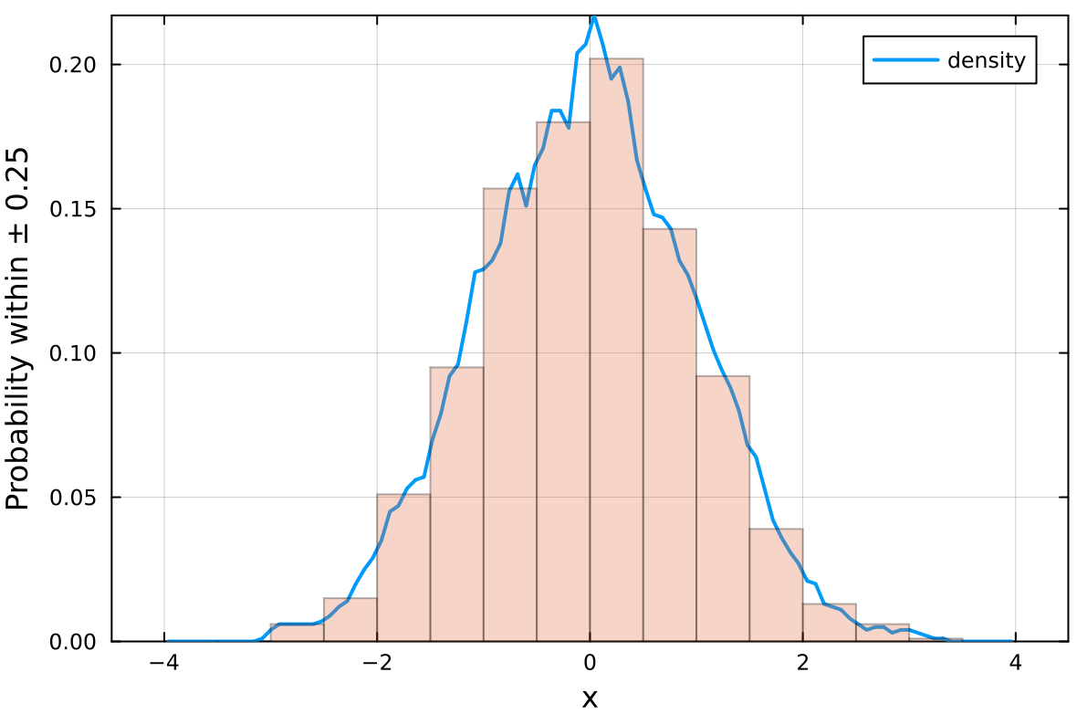
Use the fitdensity to obtain the density function (continuous histogram) of a data set x:

julia> x = randn(1000)

julia> density = fitdensity(x)

 ------------------- Density -------------

  d contains the probability of finding data points within x ± 0.25

 -----------------------------------------

Options are the step size (step=0.5) and normalization type (probability by default, with norm=1 or number of data points, with norm=0).

Example:

julia> x = randn(1000);

julia> density = fitdensity(x,step=0.5,norm=0);

julia> histogram(x,xlabel="x",ylabel="Density",label="",alpha=0.3,framestyle=:box);

julia> plot!(density.x,density.d,linewidth=2);

Bounds

Lower and upper bounds can be set to the parameters of each function using the l=lower() and u=upper() input parameters. For example:

julia> fit = fitlinear(x,y,l=lower(a=5.),u=upper(a=10.))

julia> fit = fitexp(x,y,n=2,l=lower(a=[0.,0]),u=upper(a=[1.,1.]))

Bounds to the intercepts or limiting values are not supported, but it is possible to set them to a constant value. For example:

julia> fit = fitlinear(x,y,b=5.)

julia> fit = fitexp(x,y,n=2,c=0.)

Example output:

This figure was obtained using Plots, after obtaining a fit of each type, with

julia> scatter!(x,y) # plot original data
julia> plot!(fit.x,fit.y) # plot the resulting fit

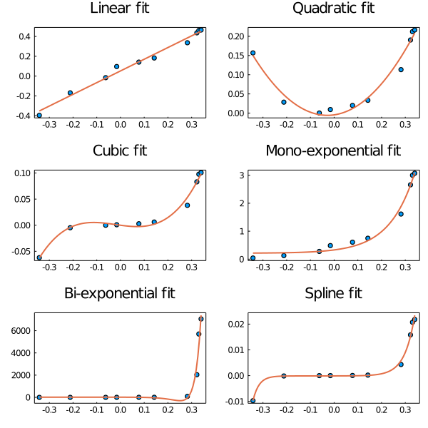
The complete script is available at: plots.jl

Options

It is possible to pass an optional set of parameters to the functions. Use, for example:

julia> fitexp(x,y,options=Options(maxtrials=1000))

Available options:

Keyword	Type	Default value	Meaning
fine	Int	100	Number of points of fit to smooth plot.
p0_range	Vector{Float64,2}	[-100*(maximum(Y)-minimum(Y)), 100*(maximum(Y)-minimum(Y))]	Range of generation of initial random parameters.
nbest	Int	5	Number of repetitions of best solution in global search.
besttol	Float64	1e-4	Similarity of the sum of residues of two solutions such that they are considered the same.
maxtrials	Int	100	Maximum number of trials in global search.
debug	Bool	false	Prints errors of failed fits.

easyfit.jl's Issues

Support for Interpolations 0.14

Current Julia versions (1.8) often build dependency trees requiring Interpolations.jl v0.14 and newer.
Would be nice to add this and trigger a release. The commands that I use (like movavg) seem wo work also with the newer Interpolations.jl version, however I did not check every function.

PS: If you're lazy I opened a PR :-)

fitpolynomial not working

@pat-alt

I merged the PR and did some code refactoring. But the polynomial fits do not seem to be working. I currently have no time to debug it, but it seems to be something related to how the model is being built. I would suggests following the same structure as the multi-exponential functions.

The tests are now in the end of the corresponding file of each type of fit. You can run them as usual, but also individually if using VScode.

Instability of fitexp

Hi,
Thank you for this very nice package!
I noticed that the exponential fit is sometimes unstable and converges to nonsense values (screenshots below).

I did not investigate further, but if needed I'd be happy to.
Best,
Pierre

Support for predictions on new values?

Neat package! Not sure if you have plans for future developments, but one thing that would be nice to have is the ability to predict from the fitted object, e.g.:

function (fit::EasyFit.Cubic)(x::Real)
    a = fit.a
    b = fit.b
    c = fit.c
    d = fit.d
    return a * x^3 + b * x^2 + c * x + d
end

Then you can just call it on new data:

julia> x = sort(rand(10)); y = x.^3 .+ rand(10);

julia> f = fitcubic(x,y)

 ------------------- Cubic Fit ----------------- 

 Equation: y = ax^3 + bx^2 + cx + d 

 With: a = 3.498571133673037
       b = -5.75292789995513
       c = 2.626129810011887
       d = 0.6361773562878126

 Pearson correlation coefficient, R = 0.7405690253097572
 Average square residue = 0.01215483592609077

 Predicted Y: ypred = [0.6416314330095221, 0.6417874373639705...
 residues = [-0.13182717628179608, -0.01592993507117535...

 ----------------------------------------------- 


julia> f.(rand(10))
10-element Vector{Float64}:
 0.8761239348448231
 0.9115358893542463
 0.9121562305431836
 0.8919530945018805
 ⋮
 0.81693749334824
 0.9622975666245418
 0.9753695182250022

TagBot trigger issue

This issue is used to trigger TagBot; feel free to unsubscribe.

If you haven't already, you should update your TagBot.yml to include issue comment triggers.
Please see this post on Discourse for instructions and more details.

If you'd like for me to do this for you, comment TagBot fix on this issue.
I'll open a PR within a few hours, please be patient!